
Human Population Genetics and Genomics ISSN 2770-5005
Human Population Genetics and Genomics 2024;4(1):0005 | https://doi.org/10.47248/hpgg2404010005
Original Research Open Access
Simulation-based benchmarking of ancient haplotype inference for detecting population structure
Jazeps Medina-Tretmanis
1

 ,
Flora Jay
2,†
,
María C. ávila-Arcos
3,†
,
Emilia Huerta-Sanchez
1,4,†
,
Flora Jay
2,†
,
María C. ávila-Arcos
3,†
,
Emilia Huerta-Sanchez
1,4,†
Correspondence: Flora Jay; María C. ávila-Arcos; Emilia Huerta-Sanchez
Academic Editor(s): Daniel Wegmann
Received: Sep 28, 2023 | Accepted: Feb 19, 2024 | Published: Mar 19, 2024
This article belongs to the Special Issue Paleogenomics, ancient DNA, and genomic tales of human history
© 2024 by the author(s). This is an Open Access article distributed under the terms of the Creative Commons License Attribution 4.0 International (CC BY 4.0), which permits unrestricted use, distribution, and reproduction in any medium or format, provided the original work is correctly credited.
Cite this article: Medina-Tretmanis J, Jay F, Ávila-Arcos M, Huerta-Sanchez E. Simulation-based benchmarking of ancient haplotype inference for detecting population structure. Hum Popul Genet Genom 2024; 4(1):0005. https://doi.org/10.47248/hpgg2404010005
Paleogenomic data has informed us about the movements, growth, and relationships of ancient populations. It has also given us context for medically relevant adaptations that appear in present-day humans due to introgression from other hominids, and it continues to help us characterize the evolutionary history of humans. However, ancient DNA (aDNA) presents several practical challenges as various factors such as deamination, high fragmentation, environmental contamination of aDNA, and low amounts of recoverable endogenous DNA, make aDNA recovery and analysis more difficult than modern DNA. Most studies with aDNA leverage only SNP data, and only a few studies have made inferences on human demographic history based on haplotype data, possibly because haplotype estimation (or phasing) has not yet been systematically evaluated in the context of aDNA. Here, we evaluate how the unique challenges of aDNA can impact phasing and imputation quality, we also present an aDNA simulation pipeline that integrates multiple existing tools, allowing users to specify features of simulated aDNA and the evolutionary history of the simulated populations. We measured phasing error as a function of aDNA quality and demographic history, and found that low phasing error is achievable even for very ancient individuals (~ 400 generations in the past) as long as contamination and average coverage are adequate. Our results show that population splits or bottleneck events occurring between the reference and phased populations affect phasing quality, with bottlenecks resulting in the highest average error rates. Finally, we found that using estimated haplotypes, even if not completely accurate, is superior to using the simulated genotype data when reconstructing changes in population structure after population splits between present-day and ancient populations. We also find that the imputation of ancient data before phasing can lead to better phasing quality, even in cases where the reference individuals used for imputation are not representative of the ancient individuals.
Keywordsancient DNA, phasing, haplotype, simulation, imputation, population structure
Unlike modern DNA, ancient DNA (aDNA) is subject to several factors that make its analysis more complicated than present-day DNA. Ancient DNA is damaged by the passage of time resulting in deamination and fragmentation [1], which makes mapping ancient reads to modern references challenging. It can also be contaminated by environmental DNA belonging to microorganisms, or modern individuals of the same species [2]. Despite this, technical and analytical advances such as next-generation sequencing (NGS) [3] and determining which substrates preserve DNA the best [4] have facilitated paleogenomics–the analysis of genomic information from ancient remains. Up to now, paleogenomic studies have contributed to (1) the development of evolutionary biology [5, 6], (2) the inference of demographic histories [7, 8], and (3) research of ancient pathogens [9].
For example, analysis of ancient human genomes from distinct time periods have been used to infer population movements [10], and these reconstructions are important to explain the genetic structure of present-day human populations. Specific examples of such studies include the characterization of migratory events in present-day Great Britain before Anglo-Saxon migrations [11], the effects of Zoroastrian migrations on the populations of Iran and India [12], genomic changes in European populations following transitions between the Stone, Bronze, and Iron ages [4], and evidence of barbarian migrations towards Italy during the 4th and 6th centuries [10].
As the availability and coverage of ancient genomes increases [13], the usage of haplotype data in paleogenomics will become more common. Considering that currently there are no benchmarks of how well phasing aDNA works as a function of contamination, average coverage and temporal drift, it is important to understand how phasing behaves when performed on aDNA data to guide studies that leverage statistical phasing [11, 12] to infer haplotypes. In general, there are three main strategies for DNA phasing. Pedigree phasing uses kinship [14] and genotype data for multiple related individuals, but it is rare to have multiple related individuals and information about how they were related in ancient data sets. Read-based phasing [14, 15] takes advantage of the fact that alleles belonging to the same read will be in phase with each other. However, the high fragmentation of aDNA makes read-based phasing difficult or computationally intractable. Finally, statistical phasing uses either a haplotype reference panel or a genotype reference cohort to determine the likeliest phasing of an individual by reconstructing the unphased individuals as a mosaic of the reference individuals. We can further split statistical phasing into reference panel phasing or population phasing [14], depending on the availability of reference haplotypes. Statistical phasing may be the only viable strategy for paleogenomic data.
Reference panel phasing makes use of a known haplotype panel, i.e., a set of high quality haplotypes that describe one or more populations. Based on this panel, the haplotypes of a new individual can be estimated by reconstructing them as a “mosaic” of the known haplotypes [16]. Three of the most used reference panels are those from the 1,000 Genomes project [17], the Haplotype Reference Consortium [18], and the TOPMed project [19]. For example, the 1,000 Genomes project gathered the haplotypes of a total of 2, 504 modern individuals belonging to 26 different populations. These populations can be divided into five super-categories: Africans, East Asians, European, South Asian, and admixed populations from the Americas [17]. This reference panel has been used in several studies in modern populations [20], as well as in studies that both phase and impute the haplotypes of ancient individuals [4, 10, 11, 12]. When no representative reference panels exist, population phasing is another strategy that does not require phased samples. Population phasing attempts to create an ad hoc reference panel by continuously updating the possible haplotypes of a cohort given only their genotypes. However, without knowledge of the underlying haplotype structure, population phasing is more computationally expensive and less accurate.
While a few studies have phased aDNA using the 1,000 Genomes reference panel, the performance of software that implements statistical phasing [16, 21] has not been evaluated for use with aDNA. Factors such as contamination, low coverage, deamination, and the time elapsed since the time of the ancient samples needs to be considered as haplotype frequencies change with time [22, 23]. Even in the best-case scenario where the reference panel individuals are direct descendants of the ancient population that is being sampled, the population might have experienced bottleneck and migration events, that together with temporal genetic drift, could decrease the reliability of phased ancient genomes.
In this study, we developed a configurable pipeline that integrates existing tools for the simulation (e.g., msprime [24], gargammel [25], seq-gen [26]) and processing of aDNA into a single software package (see Figure 1, panel A for a complete list). Our simulations account for demographic history, varying levels of contamination, damage, and coverage. We called variants on the simulated data and tested the accuracy of the haplotypes estimated by SHAPEITv2 [16], and the accuracy of imputation of missing genotypes with GLIMPSE2 [27]. We then measured how well population structure could be reconstructed from these inferred haplotypes. For each demographic scenario, we varied the age of the samples, and the divergence time between the ancient and presentday samples that are used as reference populations. Our results show that increased contamination and lower average coverages always lead to elevated phasing and imputation error. We found that when the ancient individuals belong to the same population as the reference panel individuals, and the ancient samples have a high coverage and little contamination, phasing and imputation accuracy are high. We found that population splits and bottlenecks have an effect on both phasing and imputation accuracy. We found that population phasing performs worse than reference panel phasing, and is considerably more computationally expensive. Finally, we used PCA plots on SNP matrices and ChromoPainter v2 [28] chunkcount matrices (which require phased haplotypes and indicate haplotype sharing) to evaluate whether we observed the expected structure. In summary, this work provides useful guidelines for the phasing of ancient individuals, and a tool that can be used for simulating aDNA reads under a user-specified demographic history.

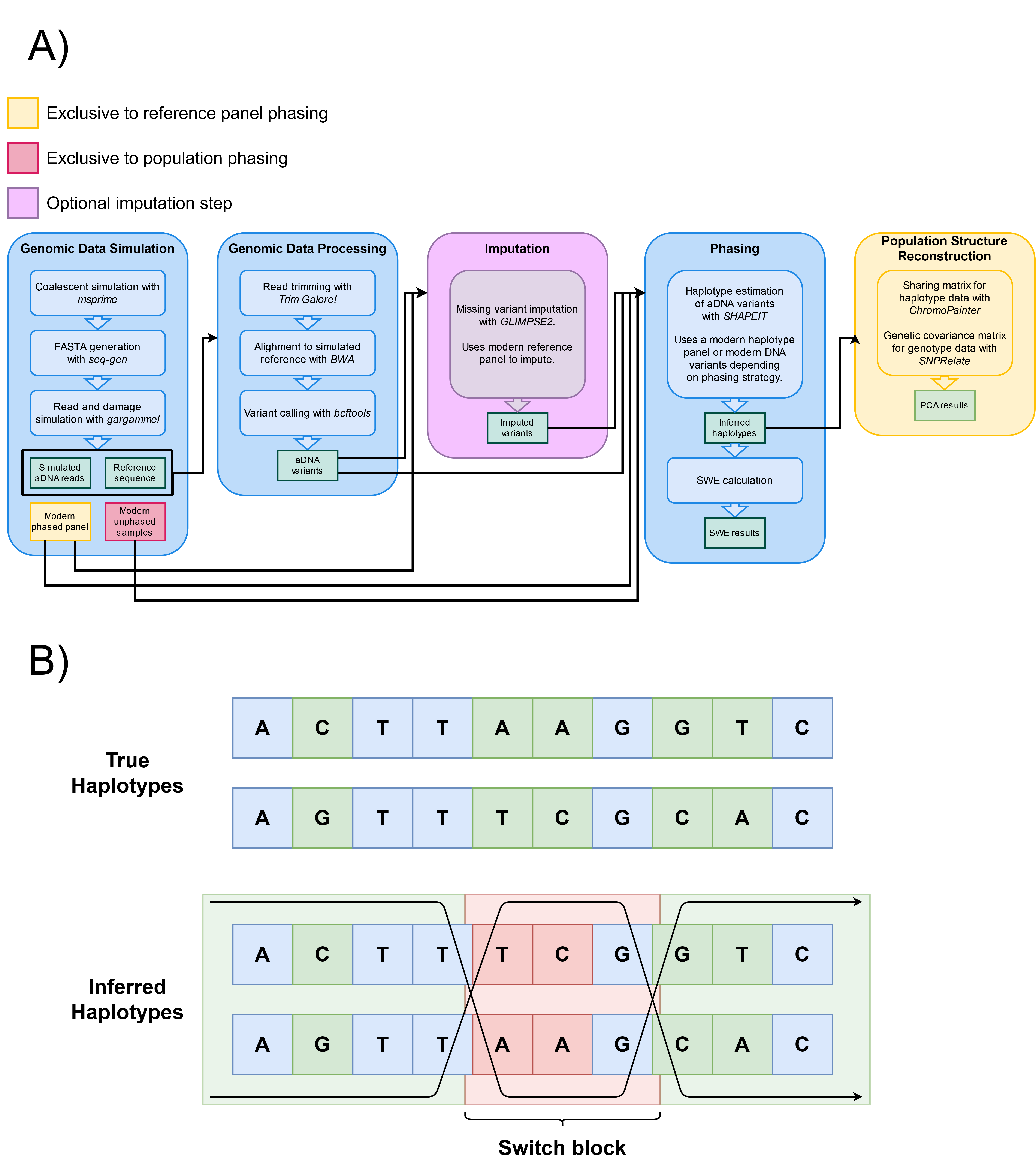
Figure 1. (A) Data simulation, processing, and analysis workflow. We consider four main stages: data simulation, processing, phasing, and population structure reconstruction. We also consider an optional imputation stage. The steps shown inside each stage list the tools required for its execution. Each stage’s execution, input, or output can vary depending on the phasing method chosen (yellow or red). SWE stands for Switch Error Rate. (B) Diagram representation of switch-errors. A switch-error is any “flip” in what the correct maternal and paternal haplotypes should be. Every switch block corresponds to two switch-errors, one for each flip. A switch-error rate is calculated as the amount of switch-errors divided by the amount of sites where a switch-error could have occurred. In this example, the phase changes two times across 5 heterozygous sites, resulting in a SWE of 40%.
We developed a pipeline to simulate ancient DNA comprising data simulation, data processing, phasing, and population structure reconstruction (Figure 1, panel A). This pipeline integrates existing tools for the simulation and processing of aDNA into a single, configurable software package. By integrating existing tools, our pipeline simulates and processes ancient DNA, it can impute and/or phase the data, and measure population structure (Figure 1, panel A). This software is available as an online GitHub repository [29].
This pipeline was developed with the intent of being as close as possible to the real workflow of a genomicist working with aDNA, specifically phasing and demographic structure reconstructions using the resulting haplotypes. The pipeline is highly parallelized, and can be easily customized by the user in different ways: the structure, history, and parameters of the simulated samples, the processing of the raw generated sequences, and the application of other methods that aren’t necessarily haplotype phasing.
To generate genomic data, we first use the coalescent simulator, msprime [24] with varying demographic models (we consider three models, see Figure 2 and Methods section 2.6) and quality parameters (see Table 2). Every simulation scenario corresponds to a unique combination of: ancient sample age, average coverage, level of contamination, and demographic scenario. For all simulation scenarios, the mutation and recombination rate were set to a value of 2×10⁻⁸ per base pair per generation. The length of the sequences was 5 MB. For each simulation scenario, we used the generated coalescent trees as input for seq-gen [26] to generate FASTA files for the ancient and present-day individuals. We generated 100 ancient and 502 present-day individuals for each simulation scenario. Of the 502 present-day individuals, one was used as the reference genome to map reads against and another one was used to introduce contamination into the ancient reads. These two individuals are from exactly the same population as the remaining 500 present-day individuals, but are not included as reference individuals in the phasing stage. The 500 remaining present-day individuals served as phased reference panel or unphased reference population for reference panel phasing or population phasing, respectively.
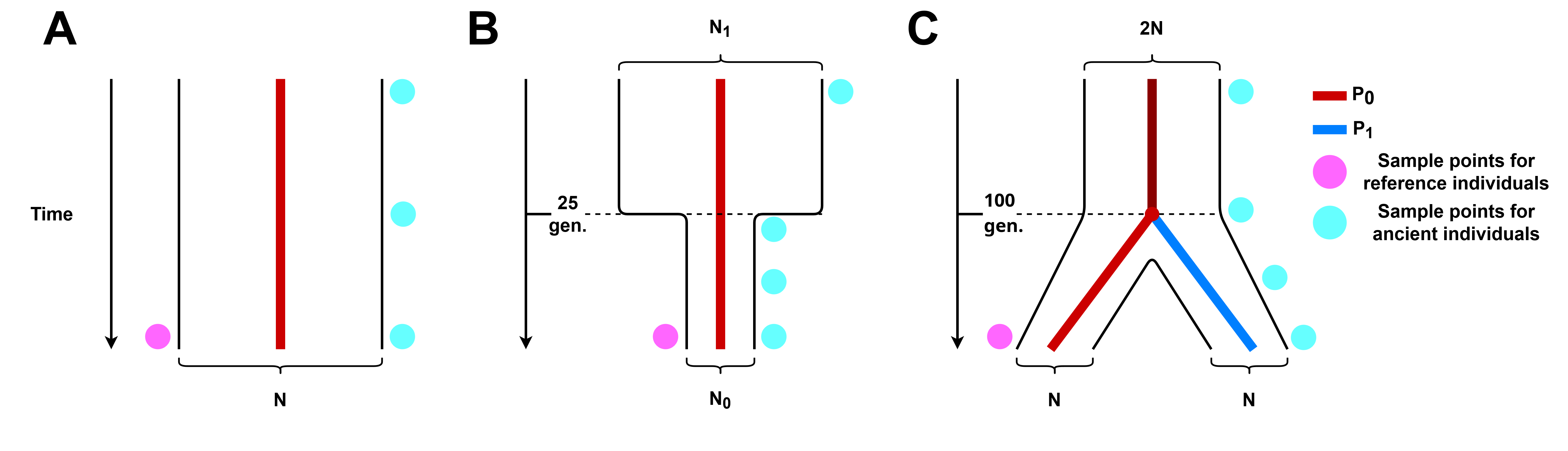
Figure 2. Simulated demographic histories. (A) No demographic events, we consider a single population P0 that remains constant in size N through time. (B) Population bottleneck.We consider a single population P0 that underwent a drastic decrease in population size 25 generations ago. (C) Population split. We consider two populations, P0 and P1, of equal size N that coalesce into a single population P0 100 generations in the past, the size of P0 previous to this time of coalescence is a constant 2N.
To generate ancient reads, we fed the 200 ancient simulated chromosomes into gargammel [25]. This tool introduces damage and fragmentation based on empirical distributions, while also simulating the desired average coverage, contamination, and sequencing errors. Table 1 shows the range for each of these parameters that result in 72 different parameter combinations. Simulated average coverages ranged from 1× to 10×, and contamination ranged from 0% to 10%. The values for coverage are illustrative of the data commonly used in aDNA studies. Depth of coverage between 1× and 10× can represent most of the data used in the previously mentioned studies [4, 10, 11, 12], and is also representative of the actual coverage of most ancient genomes sequenced [3, 30]. While most of these studies did not contain samples with modern contamination higher than 2%, we also considered values of 5% and 10% to better understand how contamination affects haplotype estimation. The damage profile of different ancient samples depends greatly on environmental factors like temperature and humidity, so it is difficult to confidently create damage profiles that correspond to different sample ages. Because of this, all samples we simulated were damaged with the same default damage matrix available in gargammel.
Table 1. Parameters for different simulated sample histories.

Simulated sequencing reads were paired-end trimmed using Trim Galore! [31] with default parameters. We then aligned the simulated reads to the simulated reference using BWA mem [32] with default parameters. After aligning all reads, we called variants using bcftools mpileup [33] and created a VCF file for each individual. Variants were filtered to have a minimum genotype quality score of 20. Considering the 5 MB length of the simulated sequences, this quality score allowed a sufficient number of variants for 1× individuals to be used in the phasing step.
Previous studies that perform statistical aDNA phasing approach this task in two ways. For example, Gnecchi-Ruscone et al. (2022) [34], used a haplotype reference panel built from modern samples to phase aDNA. On the other hand, some studies use population phasing [11, 12] by grouping the genotypes of the ancient individuals of interest with a larger number of unphased modern individuals.
We emulate these two types of phasing approaches with SHAPEITv2. For reference panel phasing we create a phased reference panel directly from the simulated sequence data of the present-day individuals (1, 000 chromosomes). In population phasing, the phases of present-day samples are ignored and inferred jointly with the phases of ancient individuals. It is much more computationally expensive since all individuals in the merged VCF must be phased.
In both cases, all ancient individuals were phased independently of each other, in other words, the phasing algorithm only had information for the reference individuals plus one specific ancient individual.
When using SHAPEITv2, it is necessary to perform an alignment step [35]. In the case of reference panel phasing, this will find the intersection of the sites in the reference panel and the sites with information available for the individual to be phased. Similarly, it will find the intersection of the sites for all individuals in the phasing cohort for population phasing. This means that if the individual to be phased has missing information for sites that are present in the reference data, these sites will be excluded completely.
Previous aDNA studies have also performed imputation of ancient genomes [4, 10, 11]. Similarly to phasing, imputation relies on the use of reference panels to find the most likely reconstructions of missing data in an unimputed individual. In order to measure the effects of sample history, quality, and age on imputation, we ran the imputation method GLIMPSE2 [27] on simulated ancient genotypes. Similarly to the phasing methodology described in section 2.3, we use the set of simulated present-day individuals as a reference panel, and perform imputation of each ancient individual independently of each other.
We followed the methodology described in the official GLIMPSE2 tutorial [36], and to measure imputation accuracy, we use the Non-Reference Discordance (NRD) metric. NRD has been used in previous studies that perform imputation on ancient data [37]. NRD is defined as the number of imputation errors divided by the number of correctly imputed heterozygous and homozygous alternate sites. That is, it ignores correctly imputed homozygous reference sites, since these sites are considerably easier to impute. NRD is negatively correlated with imputation accuracy, as a high value of NRD corresponds to lower imputation accuracy.
In order to measure the effect of imputation on haplotype phasing, we also compare the phasing accuracy of ancient individuals that underwent an imputation step prior to phasing, versus ancient individuals that were phased directly after the variant calling step. When phasing imputed individuals, we do not filter any of the imputed calls by genotype probability. We use all of the sites imputed by GLIMPSE2.
To measure phasing accuracy, we use the inferred haplotypes obtained from SHAPEITv2, and compare them to the actual haplotypes obtained from the coalescent simulation. We measure the Switch Erro rate (SWE) for each individual, which represents the amount of errors in the estimated haplotypes as a percentage (see Figure 1, panel B), specifically, the amount of sites where a phase change occurs divided by the number of sites where it could occur (heterozygous sites kept after filtering). We obtain a distribution of SWE for each different quality parameter combination.
We tested the accuracy of phasing under three simulated demographic scenarios (Figure 2): a single population of constant size through time, a single population that undergoes a bottleneck event 25 generations in the past, and the case where the modern and ancient individuals belong to two different populations that split at 100 generations in the past. All simulated parameters are listed in Table 1.
The parameters (time and effective population size change) of the bottleneck event were chosen to resemble the magnitude of the population collapse that occurred in some Native American populations due to European colonization 500 years ago [38]. For the population split, we selected a value of 100 generations in the past which is roughly 2, 500 years ago. We note that for the population split (Figure 2, panel C), the samples of the reference population are not always descendants of the ancient individuals. We did this to test the effect of using a reference population that diverged at some time in the past from the ancient individuals sampled. Considering the sample quality parameters detailed in Table 2, and demographic scenarios in Table 1, this leads to 3 demographic scenarios × 6 ancient individual ages × 4 contamination levels × 3 coverage levels = 216 different simulation scenarios. For each of these simulation scenarios we generate 500 modern individuals to serve as a reference population, 2 extra modern individuals to serve as a reference sequence and contamination source, and 100 ancient individuals to be phased for each simulation scenario. This leads to a grand total of 216 × 100 = 21, 600 phased simulated individuals.
Table 2. Tested values for each simulation quality parameter.
We employed both Principal Component Analysis (PCA) and ChromoPainter v2 for this analysis. We generated longer (20 MB) sequences, since ChromoPainter v2 expects sequences that are closer in length to a full chromosome. We only use the haplotypes inferred through reference panel phasing, as they had lower SWE and the running time for population phasing was prohibitively long for the number of replicates needed. We only considered the simulations with an average coverage of 10× and 5×, since 1× data had too few variants left after applying the quality filters specified for our variant calling step (Methods section 2.2). ChromoPainter v2 works by considering two sets of haplotypes: donors and recipients. It then uses a Hidden Markov Model to reconstruct the recipient haplotypes as a mosaic of donor haplotypes [28]. For these analyses we used the -a 0 0 option for ChromoPainter v2, which conditions all haplotypes on all other haplotypes. That is, the haplotypes of the ancient population are conditioned on both the ancient and reference haplotypes, and vice versa. The resulting chunkcounts matrix can be thought of as representing the number of segments of a given recipient haplotype that were inherited from a specific donor haplotype [28].
We tested the demographic scenario of a population split 200 generations in the past. PCA was applied to 4 different kinds of data: true genotype data (unphased SNPs), true haplotype data, genotype data called from simulated read data and the corresponding inferred haplotypes. When using genotype data, the genotype covariance matrix was built directly from the unphased VCF file using the R package, SNPRelate [39]. When using haplotype data, PCA was applied to chunkcount matrices built with ChromoPainter v2 [23] that indicate similarity between samples through counts of IBS tracts. The first and second PCs were plotted (Figure 6) and we measured how well the modern and ancient populations clustered by computing the silhouette coefficient. This metric evaluates clusterings using information inherent to the dataset, so that clustering can be compared across different simulated datasets [40]. Measuring cluster distinction is important, since distance metrics in component space can be thought of as proxies for population split times [41].
We compared the performance of population versus reference panel phasing. The lack of phased reference individuals for population phasing decreases the available information as we only have genotype information for the 500 modern individuals, this in turn increases the SWE. We simulated individuals under a bottleneck event 25 generations in the past (Figure 2, panel B), and applied population and reference panel phasing to the resulting data (Figure 3).
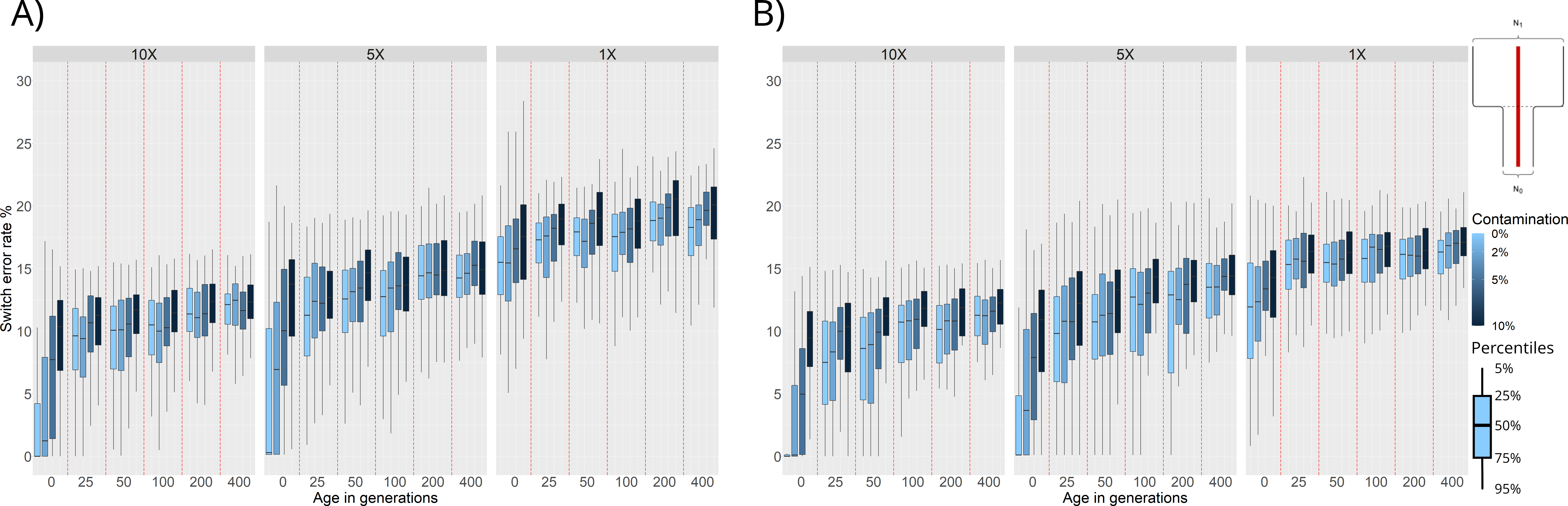
Figure 3. Switch Error Rate (SWE) distributions for phasing of ancient individuals simulated under a bottleneck event 25 generations in the past: (A) Population phasing. (B) Reference panel phasing. SWE (y-axis) is presented in 3 facets corresponding to 10×, 5×, and 1× average coverage. Within these facets are the SWE distributions for 100 simulated individuals for each combination of age (x-axis) and contamination level (shades of blue).
We find that, as expected, increasing the age and contamination or decreasing the coverage of the simulated samples results in higher SWE. Samples from before the bottleneck event (25 or more generations of age) show a high SWE (~ 10%), this can be attributed to the lack of representation of pre-bottleneck haplotypes in the post-bottleneck reference population. These trends are the same for both population and reference panel phasing, however, we can see an overall increase of SWE in the population phasing results compared to the reference panel phasing results.
Another factor to consider is running time as population phasing is more computationally expensive. SHAPEITv2’s algorithm has a time complexity of O(MJ) [16], where M is the number of SNPs to phase, and J is the number of haplotypes being conditioned on to build the likeliest phase reconstruction. Phasing a single sample with a reference panel means that J = 1, while phasing 501 individuals via population phasing means that J = 501. While execution time for phasing all data in one of our simulations using reference panels might take a couple of hours, population phasing on the same data could take upwards of 5 days depending on hardware.
We also compared the performance of population and reference panel phasing when simulating individuals under a population split event 100 generations in the past. We find similar results to the ones presented in this section, with population phasing SWE distributions being higher but following the same trends as those of their reference panel phasing counterparts (Figure S1).
Because of the increase in overall SWE when using population phasing, plus the computational complexity factors, we decided to focus on reference panel phasing results for the rest of the results.
Using reference panel phasing, we next consider the effects of demographic history on phasing accuracy. Under a constant population size, we observe an increase in SWE from ~ 1.0% — when the simulated individuals are from the present (0 generations), have high coverage and no contamination — to ~ 10.0% when increasing the age to 400 generations (Figure 4, panel A). Increasing the amount of contamination for the individuals with 0 generations of age and high coverage results in higher SWE (~ 8.0%).
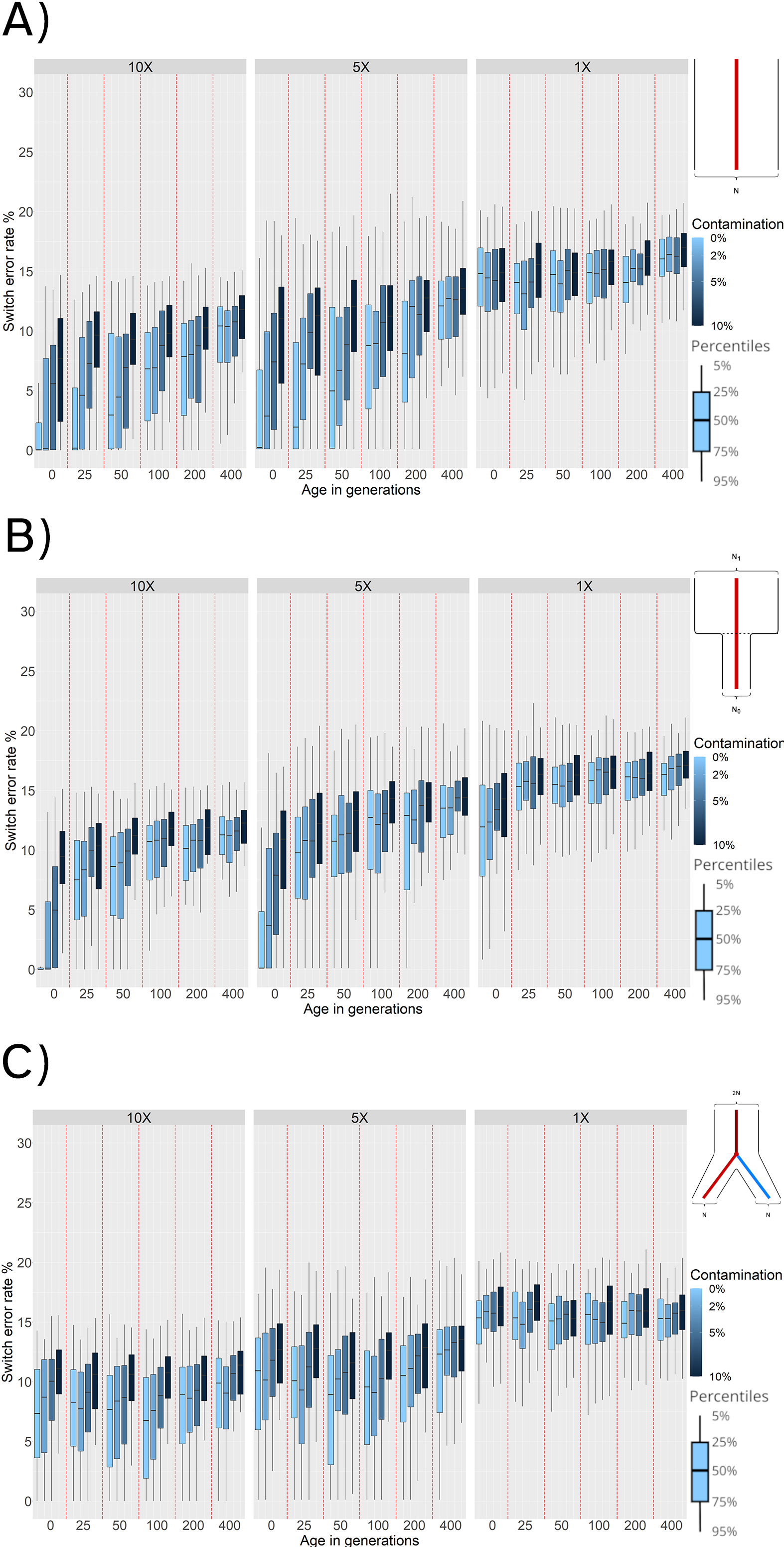
Figure 4. Switch Error Rate (SWE) distributions for reference panel phasing with: (A) Constant population scenario. (B) Bottleneck event 25 generations in the past. (C) Population split 100 generations in the past. SWE (y-axis) is presented in 3 facets corresponding to 10×, 5×, and 1× average coverage. Within these facets are the SWE distributions for 100 simulated individuals for each combination of age (x-axis) and contamination level (shades of blue).
Consistently, decreasing the average coverage from 10× to 5× results in higher SWE (~ 1.0% to ~ 6.0% for modern uncontaminated individuals across the board, and the effects of higher ages and contamination rates are preserved (Figure 4, panel A). Finally, the results for 1×average coverage showan increase in SWE across all ages and contamination rates. Within these 1× simulations, the age and contamination showlittle impact. This likely reflects that individuals sequenced at 1× have a small number of variants and some individuals are excluded because no variants pass all quality filters applied.
To test the effects of a bottleneck, we simulated a population that experienced a 90% reduction in effective population size (Ne = 10, 000 → 1, 000) 25 generations in the past (Figure 2, panel B).We find that phasing quality increases for ancient individuals that are more recent than the time of the bottleneck (0 generations of age, SWE ~ 0.3%). However, phasing quality for sampled ancient individuals older than the bottleneck event (25 generations or more) decreases. This is expected as individuals older than the time of the bottleneck belong to a population with a much higher diversity that was lost and is not captured by the modern reference individuals. Individuals with an average coverage of 1× exhibit a much higher SWE compared to results with other demographic histories (Figures 4, panels A and C), and we observe that contamination does not have a strong effect for sampled individuals that are older than the time of the bottleneck.
When we evaluate the behavior of phasing individuals of a population undergoing a split 100 generations ago from the population used as the haplotype reference panel (Figure 2, panel C), we observe that ancient individuals sampled around the time of the split (i.e., 50 to 100 generations in the past) exhibit the lowest SWE for 10× and 5× coverage values. This is expected, as samples that are more recent than the time of the split do not belong to the same population of the reference individuals (Figure 2, panel C). Therefore, both more recent and more ancient samples have higher genetic drift from the reference population than the individuals at the time of split. For sequencing coverage of 1×, the phasing quality is lower than with 5× or 10×. In the case of 1× coverage, the effect of age and contamination are negligible suggesting that coverage is the biggest factor for phasing accuracy.
We measured the effects of demographic history, age, contamination, and coverage on the imputation of simulated ancient individuals. We used GLIMPSE2 to impute the missing variants for individuals simulated under the bottleneck scenario (Figure 2, panel B). To measure imputation accuracy, we compute Non-Reference Discordance (NRD, see Methods section 2.4) after the imputation step.
Figure 5, panel A shows that NRD is higher for ancient genomes with 1× coverage than 5× or 10× coverage. This applies even when the 1× individuals are simulated under ideal conditions (0 generations of age, no contamination), with minimum NRD rates closer to ~ 8% (Figure 5, panel A). For samples with an average coverage of 10×, we observe very good imputation performance for even very ancient samples when contamination levels are low (~ 1% NRD). Increasing the levels of contamination has the biggest effect on imputation accuracy for 10× individuals, leading to NRD values closer to ~ 7.5% when contamination is at 10%. Even though ancient samples with a coverage of 10× would normally not be imputed, we can still see benefits in terms of phasing accuracy when imputing these individuals (Figure 5, panel C).
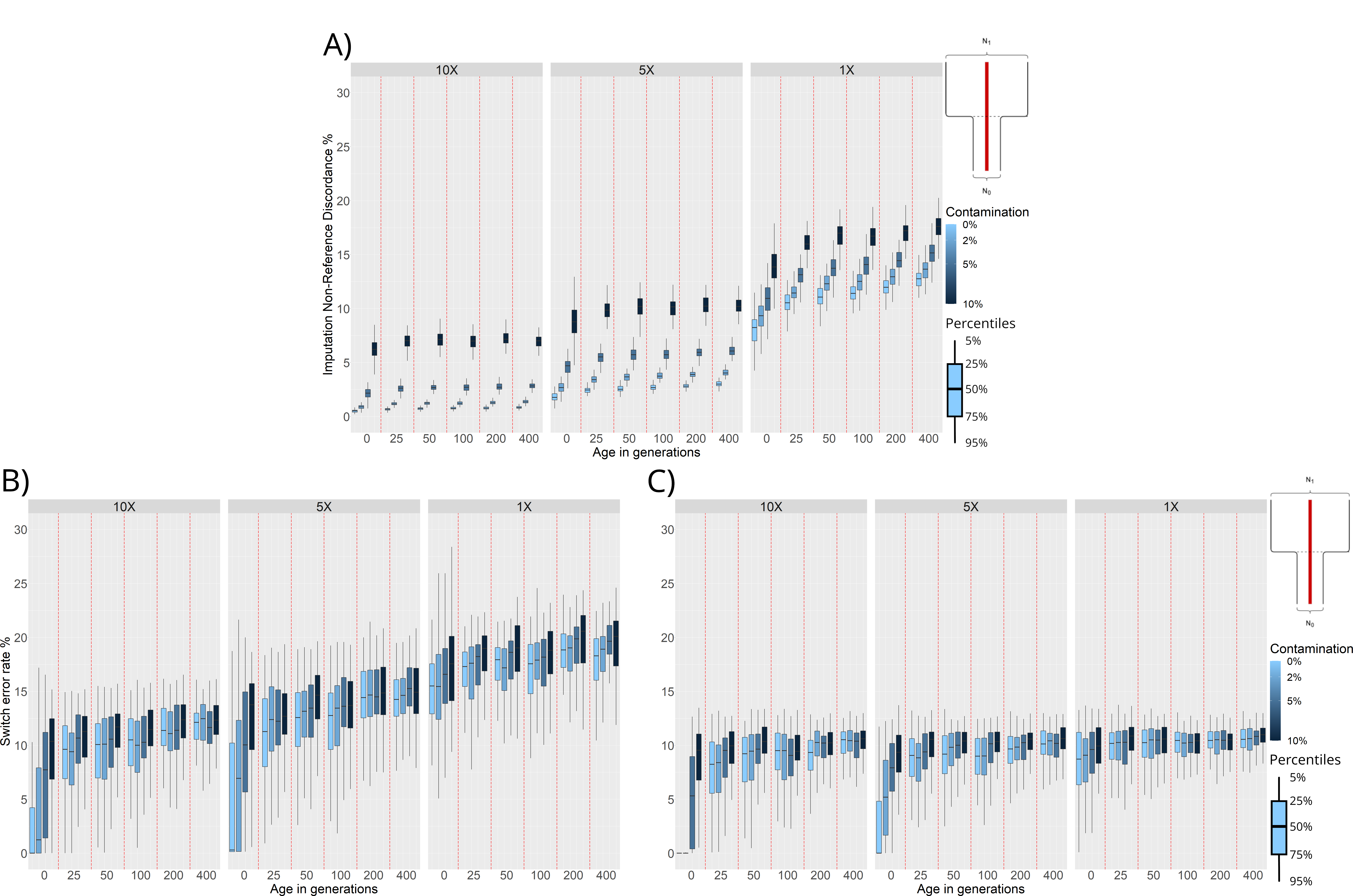
Figure 5. Non-Reference Discordance (NRD) and Switch Error Rate (SWE) distributions for individuals simulated under a demographic model with a bottleneck event 25 generations in the past. NRD or SWE (y-axis) are presented in facets corresponding to 10×, 5×, and 1× average coverage. For each combination of age (x-axis) and contamination level (shades of blue), we plot the distributions of NRD and SWE values computed for each of the 100 simulated individuals. All phasing results were obtained through reference panel phasing. (A) NRD distributions of imputed variants. (B) SWE distributions of unimputed individuals. (C) SWE distributions of imputed individuals.
For lower coverage individuals (5× and 1×) we see a much more important effect of age on imputation performance. In these cases, there is a noticeable increase in NRD when imputing individuals from before the time of the bottleneck. Again, this is expected, as the reference panels used for imputation are not representative of the haplotypic diversity present in the population before the bottleneck occurred (Figure 5, panel A).
To assess whether imputing ancient genomes before phasing leads to better phasing accuracy, we compared the phasing performance on the unimputed and imputed ancient individuals in the bottleneck scenario (Figure 5, panels B and C). As explained in section 3.2, when we phase unimputed individuals simulated under the bottleneck scenario (Figure 2, panel B), we can see a marked increase in phasing error for individuals from before the time of the bottleneck (Figure 4, panel B). When we first impute and then phase the individuals this same trend remains. However, imputing the individuals before phasing leads to a dramatic decrease in overall phasing error for all coverages (see Figure 5, panels B and C). For example, Figure 5, panel C shows that SWE decreases by ~ 7% for imputed 1× individuals compared to unimputed 1× individuals. While imputation greatly improves the SWE in low coverage individuals, we still find that the SWE of imputed 10× and 5× individuals is markedly lower (~ 0% vs. ~ 8%) when the individuals are sampled after the bottleneck (i.e., 0 generations of age).
We also measured imputation and phasing accuracy under the population split scenario (Figure 2, panel C). Similarly as before, we computed NRD and compared the phasing accuracy of imputed and unimputed individuals. We observe similar trends to the ones presented under the bottleneck scenario, with the phasing of imputed individuals displaying lower SWE distributions than their unimputed counterparts (Figure S2).
We further tested if population structure could be accurately recovered from inferred haplotypes, and how much of an impact would haplotype estimation error have on these reconstructions. To do this, we simulated samples under a population split model with a population split 200 generations ago (Figure 2, panel C), and sequence length of 20 MB. We sampled 100 ancient individuals 25 generations ago and 500 present-day reference individuals. We note that the ancient samples and reference samples do not belong to the same population in this scenario (Figure 2, panel C). To test if population structure was visually recoverable, we plotted the first and second Principal Components (PCs) obtained by running PCA on four different kinds of data resulting from this simulated demographic history. Note that in this context, true refers to the exact outputs of the coalescent simulations: (1) the true genotypes, (2) the true haplotypes, (3) genotype data called from the sequencing reads generated with damage, contamination (0-10%) and two average coverage levels (5×, 10×) and (4) the inferred haplotypes using reference panel phasing on the called genotypes from (3). (1) and (2) refer to the base truth for genotypes and haplotypes, and (3) and (4) refer to the genotypes and haplotypes that are obtained after simulating damage and quality parameters. We applied PCA to the genotype matrices ((1) and (3)) or to the chunkcount matrices obtained from ChromoPainter v2[23] based on haplotype data ((2) and (4); see Methods section 2.7).
Using either the true genotype data (Figure 6, panel A), or the true haplotype data (Figure 6, panel B), PCA reveals distinct clusters for modern reference and ancient samples, which is expected given that they belong to two distinct populations. The clusters are more distinct when recovered from the true haplotype data.
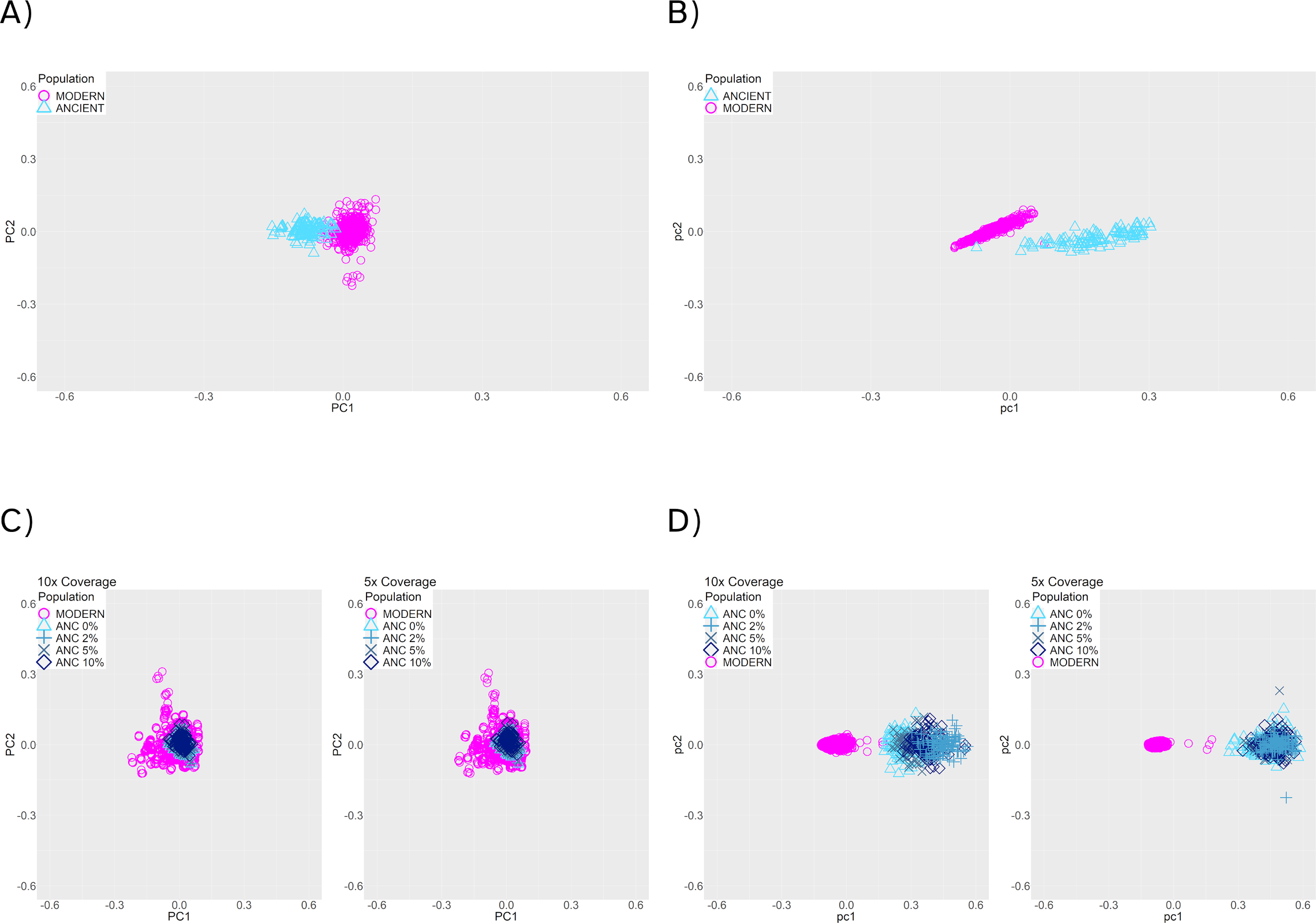
Figure 6. PCA of modern (pink) and 25-generation-old individuals (blue), with a population split 200 generations in the past. (A) True genotype matrix (1). (B) True haplotype data (2). (C) Called genotype data. (3) (D) Estimated haplotypes from the called genotype data (4). Panels (C) and (D) show results with 10× (left) and 5× (right) coverage, and 0% to 10% contamination rates (blue symbols).
When using genotype data after applying damage, contamination, and missingness to the simulated data (3), the first two PCs no longer recover population structure (Figure 6, panel C). In contrast, the haplotypes recovered after reference panel phasing render a visually recognizable separation between the clusters (Figure 6, panel D), suggesting that using haplotype data provides better resolution. From this, we conclude that the current phasing procedure enables the recovery of population structure from ancient haplotype data, despite the noise present in aDNA.
Silhouette coefficients offer a way of measuring and comparing the clustering performance for these four kinds of data, independently of the fact that each PCA was done on a different set of data. These coefficients can range from -1 to 1, with values closer to 1 indicating better clustering performance. We found that silhouette coefficients for the PCAs on genotype data (coefficient for (1): 0.499, coefficient for (3): -0.131) were substantially lower than those for the PCAs on haplotype data (coefficient for (2): 0.729, coefficient for (4): 0.920). Since the clustering is much more distinct in (4) compared to (3), this suggests that the extra information present in the haplotype sharing matrices that ChromoPainter v2 outputs is better for differentiating the population structure of the modern and ancient individuals with a split 200 generations in the past, at least when compared to using only genotypes.
Using haplotype data can be powerful to infer demographic history. While it is common to use haplotype data to infer the demographic history of a population using present-day genomes, only a few studies have phased ancient genomes. In this study, we have developed a pipeline to simulate ancient read sequencing data to benchmark phasing of aDNA as a function of different parameters. Specifically, we show how phasing quality changed as we varied coverage, contamination, temporal drift and population split times. We also examined how these parameters affected levels of observable population structure as captured by PCA and ChromoPainter v2.
We first benchmarked the accuracy of population phasing and reference panel phasing. As our results show that reference-panel phasing is more accurate (using measures of Switch Error Rate, SWE) and faster than population phasing (Results section 3), most of the benchmarking analyses performed in this study consider reference panel phasing. When we measured phasing accuracy as a function of coverage, we find that decreasing the average coverage leads to higher SWE; since having less SNPs available for the statistical phasing algorithm reduces the certainty at which phase can be inferred (see Figure 4, panel B), and in general, sample coverage has the strongest effect on phasing accuracy. Also, as contamination increases, the phasing quality decreases regardless of whether we used reference panel phasing or population phasing (Figure 3). This makes sense as introducing new variants via contamination will affect the probability distribution of haplotypes estimated by SHAPEITv2, and contamination levels as high as 10% introduce more false variants than any other kinds of damage. In this work, we only included contamination from individuals that belonged to the same population as the reference population. However, it is unclear how other contamination scenarios would affect phasing. For example, considering scenarios like contamination from individuals not closely related to either the reference or ancient populations may lead to higher phasing errors, and might be a valuable avenue of research for future work.
To assess the effects of temporal drift, we sampled ancient genomes at different times in the past. Increasing the age of the simulated ancient individuals directly increases the SWE in the phased haplotypes. This occurs when we simulate either a constant population size or when we simulate bottlenecks (Figure 4, panels A and B). We find that low phasing error rates can be obtained from very ancient individuals if we have good quality samples (average coverage over 5× and contamination below 5%), and reference panels that are representative of the ancient individual. This is most apparent when no demographic changes through time are simulated, thus ensuring more continuity between the reference and phased populations (Figure 4, panel A).
We find that population bottlenecks increase SWE, especially when the sampling time of the ancient individuals is equal to or greater than the time of the bottleneck. This is probably happening because bottlenecks result in a loss of genetic and haplotype variation. Therefore, haplotype inference for ancient individuals older than the time of bottleneck will always result in a low phasing quality (mean SWE of at least 7.5%), independently of other sample parameters.
Under demographic models with population splits, the behavior of phasing error is different. The lowest error rates (Figure 4, panel C) occur when the sampling time of the ancient individuals is closest to the time of the population split. This implies that older samples do not necessarily lead to worse phasing accuracy, but rather genetic distance from individuals in the reference populations. In other words, when we simulated population splits, we found that proximity to the reference population was the most important factor in terms of sample age. This is expected for two reasons: individuals with a more recent age than the time of the split belong to a population that is increasingly divergent from the reference population. Conversely, individuals that are older than the time of split belong to the ancestral population of the reference individuals, but increasing the age further results in more temporal drift that leads to a higher SWE (Figure 4).
Recent studies have suggested that using present-day reference panels may be a good strategy to impute missing genotypes in ancient individuals [37]. Here, we measured imputation accuracy under two demographic scenarios (Figure 5, Figure S2), and we also measured phasing accuracy after first imputing ancient genomes. We found that the quality of imputation and phasing are affected by demographic history, sample age, contamination, and coverage in similar ways (Figure 5, panel A, Figure S2, panel A). For example, under a population bottleneck scenario, we find that imputing individuals from before the time of the bottleneck leads to higher imputation error. Imputing before phasing, however, always reduces phasing error for all simulated parameters in the bottleneck and population split demographic scenarios (Figure 5, Figure S2). This can be attributed to the increase in data available to the phasing algorithm compared to phasing unimputed individuals. Even though imputation of ancient individuals is imperfect, we find that a large portion of sites are correctly imputed even under the worst quality conditions simulated (Figure 5). Consequently, the increase in sites used as input for the phasing algorithm overall improves the phasing quality. This suggests that imputing ancient individuals is a good preprocessing step when phasing aDNA.
We also assess the implications of phasing ancient individuals in the context of population structure. We find that we can recapitulate the population structure with the inferred haplotypes, and that it is better than using only genotype data (Figure 6, panel D). Parameters such as contamination and coverage slightly affect clustering, but even in those cases we recover population structure (Figure 6).
In this work, we provide the first study (to our knowledge) that benchmarks phasing in aDNA while accounting for various features of the data such as age, contamination, coverage, and demographic history. Although we simulated only a subset of possible data quality parameters and demographic scenarios, these results are a good starting point for guiding future studies that necessitate aDNA phasing. While pieces of the pipeline already exist (e.g., sequence [26] and read [25] simulation), here we provide an easy to install and open source software that streamlines all steps from simulation under a demographic model to visualization which will be helpful for others to evaluate how phasing quality might be affected by characteristics specific to other systems or populations.
The following supplementary materials are available at: HPGG2404010005SupplementaryMaterials.zip
Figure S1. Switch Error Rate (SWE) distributions for phasing of ancient individuals simulated under a population split 100 generations in the past.
Figure S2. Non-Reference Discordance (NRD) and Switch Error Rate (SWE) distributions for individuals simulated under a demographic model with a population split event 100 generations in the past. NRD or SWE (y-axis) are presented in facets corresponding to 10×, 5×, and 1× average coverage.
Not applicable.
Not applicable.
All software used for simulation and analysis is available at github.com/Jazpy/Paleogenomic-Datasim.
This work was supported by the PAPIIT program offered by UNAM-DGAPA with filing number IA203821, by grant CN 17-12 of the UC MEXUS-Conacyt program, by the Alfred P. Sloan Award, by a Young Investigator’s grant from the Human Frontier Science Program, by NIH grant R35GM128946, and by grant ANR-20-CE45-0010-01 RoDAPoG.
The authors have declared that no competing interests exist.
Conceptualization, María C. Ávila-Arcos and Emilia Huerta-Sanchez; Methodology, Jazeps Medina-Tretmanis, Flora Jay, María C. Ávila-Arcos and Emilia Huerta-Sanchez; Software, Jazeps Medina-Tretmanis; Validation, Jazeps Medina-Tretmanis, Flora Jay, María C. Ávila-Arcos and Emilia Huerta-Sanchez; Formal Analysis, Jazeps Medina-Tretmanis; Investigation, Jazeps Medina-Tretmanis; Resources, Jazeps Medina-Tretmanis; Data Curation, Jazeps Medina-Tretmanis; Writing – Original Draft Preparation, Jazeps Medina-Tretmanis; Writing – Review & Editing, Jazeps Medina-Tretmanis, Flora Jay, María C. Ávila-Arcos and Emilia Huerta-Sanchez; Visualization, Jazeps Medina-Tretmanis; Supervision, Flora Jay, María C. Ávila-Arcos and Emilia Huerta-Sanchez; Project Administration, Flora Jay, María C. Ávila-Arcos and Emilia Huerta-Sanchez; Funding Acquisition, Flora Jay, María C. Ávila-Arcos and Emilia Huerta-Sanchez.
This work received support from Luis Aguilar, Alejandro De León, and Jair García of the Laboratorio Nacional de Visualización Científica Avanzada. This research was conducted using computational resources and services at the Center for Computation and Visualization, Brown University. Special thanks to the Huerta-Sanchez and Ávila-Arcos labs for continued feedback and support.
| 1. | Prüfer K, Stenzel U, Hofreiter M, Pääbo S, Kelso J, Green RE. Computational challenges in the analysis of ancient DNA. Genome Biol. 2010;11(5):R47. [Google Scholar] [CrossRef] |
| 2. | Burger J, Hummel S, Herrmann B, Henke W. DNA preservation: A microsatellite-DNA study on ancient skeletal remains. Electrophoresis. 1999;20(8):1722-1728. [Google Scholar] [CrossRef] |
| 3. | Knapp M, Hofreiter M. Next Generation Sequencing of Ancient DNA: Requirements, Strategies and Perspectives. Genes. 2010;1(2):227-243. [Google Scholar] [CrossRef] |
| 4. | Gamba C, Jones ER, Teasdale MD, McLaughlin RL, Gonzalez-Fortes G, Mattiangeli V, et al. Genome flux and stasis in a five millennium transect of European prehistory. Nat Commun. 2014;5:5257. [Google Scholar] [CrossRef] |
| 5. | Pont C, Wagner S, Kremer A, Orlando L, Plomion C, Salse J. Paleogenomics: reconstruction of plant evolutionary trajectories from modern and ancient DNA. Genome Biol. 2019;20(19):29. [Google Scholar] [CrossRef] |
| 6. | Shapiro B, Hofreiter M. A paleogenomic perspective on evolution and gene function: new insights from ancient DNA. Science. 2014;343(6169):1236573. [Google Scholar] [CrossRef] |
| 7. | Skoglund P, Mathieson I. Ancient genomics of modern humans: the first decade. Annu Rev Genomics Hum Genet. 2018;19(1):381-404. [Google Scholar] [CrossRef] |
| 8. | Llamas B, Fehren-Schmitz L, Valverde G, Soubrier J, Mallick S, Rohland N, et al. Ancient mitochondrial DNA provides high-resolution time scale of the peopling of the Americas. Sci Adv. 2016;2(4):e1501385. [Google Scholar] [CrossRef] |
| 9. | Spyrou MA, Bos KI, Herbig A, Krause J. Ancient pathogen genomics as an emerging tool for infectious disease research. Nat Rev Genet. 2019;20(6):323-340. [Google Scholar] [CrossRef] |
| 10. | Amorim CEG, Vai S, Posth C, Modi A, Koncz I, Hakenbeck S, et al. Understanding 6th-century barbarian social organization and migration through paleogenomics. Nat Commun. 2018;9(1):3547. [Google Scholar] [CrossRef] |
| 11. | Martiniano R, Caffell A, Holst M, Hunter-Mann K, Montgomery J, Müldner G, et al. Genomic signals of migration and continuity in Britain before the Anglo-Saxons. Nat Commun. 2016;7:10326. [Google Scholar] [CrossRef] |
| 12. | López S, Thomas MG, van Dorp L, Ansari-Pour N, Stewart S, Jones AL, et al. The genetic legacy of Zoroastrianism in Iran and India: insights into population structure, gene flow, and selection. Am J Hum Genet. 2017;101(3):353-368. [Google Scholar] [CrossRef] |
| 13. | Callaway E. ‘Truly gobsmacked’: Ancient-human genome count surpasses 10,000. Nature. 2023;617:20. [Google Scholar] [CrossRef] |
| 14. | Choi Y, Chan AP, Kirkness E, Telenti A, Schork NJ. Comparison of phasing strategies for whole human genomes. PLoS Genet. 2018;14(4):e1007308. [Google Scholar] [CrossRef] |
| 15. | Martin M, Patterson M, Garg S, Fischer SO, Pisanti N, Klau GW, et al. WhatsHap: fast and accurate read-based phasing. bioRxiv. 2016;495S. [Google Scholar] [CrossRef] |
| 16. | Delaneau O, Marchini J, Zagury JF. A linear complexity phasing method for thousands of genomes. Nat Methods. 2012;9:179-181. [Google Scholar] [CrossRef] |
| 17. | The 1000 Genomes Project Consortium, Auton A, Brooks LD, Durbin RM, Garrison EP, Kang HM, et al. A global reference for human genetic variation. Nature. 2015;526(7571):68-74. [Google Scholar] [CrossRef] |
| 18. | McCarthy S, Das S, Kretzschmar W, Delaneau O, Wood AR, Teumer A, et al. A reference panel of 64,976 haplotypes for genotype imputation. Nat Genet. 2016;48(10):1279-1283. [Google Scholar] [CrossRef] |
| 19. | Das S, Forer L, Schönherr S, Sidore C, Locke AE, Kwong A, et al. Nextgeneration genotype imputation service and methods. Nat Genet. 2016;48(10):1284-1287. [Google Scholar] [CrossRef] |
| 20. | Birney E, Soranzo N. The end of the start for population sequencing. Nature. 2015;526(7571):52-53. [Google Scholar] [CrossRef] |
| 21. | Browning SR, Browning BL. Rapid and accurate haplotype phasing and missing-data inference for whole-genome association studies by use of localized haplotype clustering. Am J Hum Genet. 2007;81(5):1084-1097. [Google Scholar] [CrossRef] |
| 22. | Sabeti PC, Reich DE, Higgins JM, Levine HZP, Richter DJ, Schaffner SF, et al. Detecting recent positive selection in the human genome from haplotype structure. Nature. 2002;419(6909):832-837. [Google Scholar] [CrossRef] |
| 23. | Lawson DJ, Hellenthal G, Myers S, Falush D. Inference of population structure using dense haplotype data. PLoS Genet. 2012;8(1):e1002453. [Google Scholar] [CrossRef] |
| 24. | Kelleher J, Etheridge AM, McVean G. Efficient coalescent simulation and genealogical analysis for large sample sizes. PLoS Comput Biol. 2016;12(5):e1004842. [Google Scholar] [CrossRef] |
| 25. | Renaud G, Hanghøj K, Willerslev E, Orlando L. gargammel: a sequence simulator for ancient DNA. Bioinformatics. 2017;33(4):577-579. [Google Scholar] [CrossRef] |
| 26. | Rambaut A, Grassly NC. Seq-Gen: An application for the Monte 520 Carlo simulation of DNA sequence evolution along phylogenetic trees. Comput Appl Biosci. 1997;13(3):235-238. [Google Scholar] [CrossRef] |
| 27. | Rubinacci S, Hofmeister RJ, Sousa da Mota B, Delaneau O. Imputation of low-coverage sequencing data from 150,119 UK Biobank genomes. Nat Genet. 2023;55(7):1088-1090. [Google Scholar] [CrossRef] |
| 28. | Hellenthal G. Instruction manual for “ChromoPainter: a copying model for exploring admixture in population data” [Internet]. 2012. Available from: https://people.maths.bris.ac.uk/madjl/finestructure-old/ChromoPainterInstructions.pdf. |
| 29. | Implementation of the described pipeline [Internet]. Available from: https://github.com/Jazpy/Paleogenomic-Datasim. |
| 30. | Ausmees K, Sanchez-Quinto F, Jakobsson M, Nettelblad C. An empirical evaluation of genotype imputation of ancient DNA. G3. 2022;12(6):jkac089. [Google Scholar] [CrossRef] |
| 31. | Krueger F. Trim Galore! [Internet]. Available from: https://github.com/FelixKrueger/TrimGalore. |
| 32. | Li H, Durbin R. Fast and accurate short read alignment with Burrows-Wheeler Transform. Bioinformatics. 2009;25(14):1754-1760. [Google Scholar] [CrossRef] |
| 33. | Li H, Handsaker B, Wysoker A, Fennell T, Ruan J, Homer N, et al. The sequence alignment/map format and SAMtools. Bioinformatics. 2009;25(16):2078-2079. [Google Scholar] [CrossRef] |
| 34. | Gnecchi-Ruscone GA, Szécsényi-Nagy A, Koncz I, Csiky G, Rácz Z, Rohrlach AB, et al. Ancient genomes reveal origin and rapid trans-Eurasian migration of 7th century Avar elites. Cell. 2022;185(8):1402-1413.e21. [Google Scholar] [CrossRef] |
| 35. | SHAPEITv2 Manual [Internet]. Available from: https://mathgen.stats.ox.ac.uk/genetics_software/shapeit/shapeit.html. |
| 36. | Getting started [Internet]. Available from: https://odelaneau.github.io/GLIMPSE/docs/tutorials/getting_started/. |
| 37. | da Mota BS, Rubinacci S, Cruz Dávalos DI, Amorim CEG, Sikora M, Johannsen NN, et al. Imputation of ancient human genomes. Nat Commun. 2023;14(1):3660. [Google Scholar] [CrossRef] |
| 38. | Acuna-Soto R, Stahle DW, Cleaveland MK, Therrell MD. Megadrought and Megadeath in 16th Century Mexico. Emerg Infect Dis. 2002;8(4):360-362. [Google Scholar] [CrossRef] |
| 39. | Zheng X, Levine D, Shen J, Gogarten SM, Laurie C, Weir BS. A high-performance computing toolset for relatedness and principal component analysis of SNP data. Bioinformatics. 2012;28(24):3326-3328. [Google Scholar] [CrossRef] |
| 40. | Rousseeuw PJ. Silhouettes: A graphical aid to the interpretation and validation of cluster analysis. J Comput Appl Math. 1987;20:53-65. [Google Scholar] [CrossRef] |
| 41. | McVean G. A Genealogical Interpretation of Principal Components Analysis. PLoS Genet. 2009;5(10):e1000686. [Google Scholar] [CrossRef] |

![]()
Copyright © 2026 Pivot Science Publications Corp. - unless otherwise stated | Terms and Conditions | Privacy Policy


