Human Population Genetics and Genomics ISSN 2770-5005

Human Population Genetics and Genomics 2025;5(4):0008 | https://doi.org/10.47248/hpgg2505040008

Original Research Open Access

The Quantitative Genetics of Human Disease: 3A Interactions—Correlation in State

Kiana Jodeiry 1,2 , Andrew J. Bass 2,3,† , Michael P. Epstein 2,3 , David J. Cutler 2,3

  • Department of Psychology, Emory University, Atlanta, Georgia 30322, USA
  • Center of Computational and Quantitative Genetics, Emory University, Atlanta, Georgia 30322, USA
  • Department of Human Genetics, Emory University,Atlanta, Georgia 30322, USA
  • Current address: Department of Medicine, University of Cambridge, Addenbrooke’s Hospital, Hills Road, Cambridge, UK

Correspondence: David J. Cutler

Academic Editor(s): Carina Schlebusch, Lounès Chikhi

Received: Oct 30, 2024 | Accepted: Dec 19, 2025 | Published: Dec 26, 2025

© 2025 by the author(s). This is an Open Access article distributed under the Creative Commons License Attribution 4.0 International (CC BY 4.0) license, which permits unrestricted use, distribution and reproduction in any medium or format, provided the original work is correctly credited.

Cite this article: Jodeiry K, Bass AJ, Epstein MP, Cutler DJ. The Quantitative Genetics of Human Disease: 3A Interactions—Correlation in State. Hum Popul Genet Genom 2025; 5(4):0008. https://doi.org/10.47248/hpgg2505040008

Abstract

The third section of an anticipated four paper series distinguishes two different forms of genetic interactions. In this, the first paper of our discussion on genetic interactions, we describe interactions arising from correlation between genotypic and/or environmental states. In the second paper, we will describe interactions arising from non-additivity between uncorrelated factors (epistasis). We illustrate the ways in which correlations in allelic and genotypic state dramatically alter our intuitions and our quantitative genetic estimates, demonstrating why they must be explicitly accounted for. Departures from Hardy-Weinberg equilibrium are understood as a form of interaction caused by correlations in allelic state within a locus. We review the effects of ancestry on correlation in state within a locus and correlation in state between loci (linkage disequilibrium), with the latter contributing to test statistic inflation in association studies. Relatedness is understood as correlation in allelic state due to recent ancestry. Here we show that population structure, i.e., ancestry, is most simply understood as causing correlation in state between factors, and we demonstrate methods to estimate quantitative genetics quantities while accounting for the correlation in state of alleles induced by complex ancestry.

Keywords

quantitative genetics, human disease, genetic interactions, population structure, linkage disequilibrium

1. Introduction

At its essence, the goal of human genetics is to discover genes that causally influence disease initiation or progression. At the genome-wide scale, case-control association studies approach this goal by identifying statistical relationships (i.e., correlations) between single nucleotide polymorphisms (SNPs) and disease status. The simplest possible analytic strategies for performing association studies often assume the data have the property of being identical and independently distributed (although there are many more recent strategies for considering the joint effects of multiple variants in a region on phenotype [1-4]). The simplest approach assumes each random variable (in this context, genotypes at SNPs) is mutually independent, sharing the same probability distribution with other variables, and correlations in the state of genotypes is usually treated as some sort of confounding to be "removed".

When conducting GWAS and fine-mapping association studies, researchers often seek to reduce the influence of factors frequently viewed as artifacts: departures from Hardy-Weinberg Equilibrium (HWE), linkage disequilibrium, population structure, and relatedness among the individuals under study. These factors are usually viewed as departures from model assumptions that can bias test statistics or parameter estimation. While this view is certainly true and often extremely useful, here we will view all of these elements as related manifestations of the same phenomena, correlation in state between genetic factors. Departures from Hardy-Weinberg equilibrium are understood as a form of interaction caused by correlation in allelic state within a locus. Linkage disequilibrium is understood as correlation in allelic state between different loci. Relatedness is understood as correlation in allelic state due to recent ancestry. Complex ancestry over many generations (population structure) is understood from its effects on correlation in state within and between loci. Population structure refers to the presence of subgroups of individuals in the sample under study, such as subgroups with different ancestral backgrounds, who differ systematically across loci in their allele frequencies. In this paper, we demonstrate how variation in ancestry can create correlation in allelic state between every site in the genome, violating the assumption of independence of genetic factors, and acting as the fundamental cause of GWAS test statistic inflation. From our perspective, we will view the effects of population structure on genetic association studies as a form of interaction created by correlations in genotypic state, later contrasting it with non-additive interactions between uncorrelated markers (epistasis) in the second paper of our discussion of interactions [5].

2. Materials and Methods

We begin with a reminder [6] of our Kempthorne [7] inspired definition of "effect". The effect of being in any particular state of some factor, or any collection of states, is defined to be the average phenotype of individuals who are in that state or collection of states. The effect of an A1A_1 allele is the average phenotype of individuals who possess the A1A_1 allele. The effect of the combination of the A1A_1 allele and environmental state e1e_1 is the average phenotype of individuals who have the combination of the A1A_1 allele along with environmental state e1e_1. An interaction is said to exist whenever the effect of a combination of states is not equal to the sum of the individual state effects. It is helpful to distinguish two forms of interaction. Interactions can arise from correlation in the state of two factors, i.e., the chance of having allele A1A_1 might be correlated with the chance of being in environmental state e1e_1—these are the interactions discussed in this paper. Alternatively, the state of factors might be independent, but the effect of two or more factor states is different from the sum of the individual state effects: the independent factors are "non-additive"—we discuss these interactions in the next paper of this series [5]. When the two factors are both genetic, correlation in genetic state is often called "linkage disequilibrium" when considering allelic states at two different loci and "population structure" when considering allelic states within a locus, but these terms are far from consistently applied or used.

We find it important to distinguish correlation in state from non-additivity of independent factors, because the results of these two forms of interaction can be vastly different. Non-additivity among independent factors does not change individual effect sizes, but always increases the total variance. Correlation in state is far more complex and can cause changes in individual state effects (changes in means) as well as increases or even decreases in the total variance relative to the sum of the individual state variances. We first encountered this when examining linkage disequilibrium (LD)—the correlation in genotypic state between two different SNPs—where we observed LD to change the mean effects of individual alleles and make the total genetic variance less than the sum of the individual locus variances [6].

Departures from Hardy-Weinberg equilibrium

The first paper in this series [6] attempted to derive major quantitative genetics results with as few assumptions as possible, yet throughout the entirety of that presentation, one major assumption remained: Hardy-Weinberg Equilibrium (HWE). We chose to embrace HWE because it greatly simplified an already complex presentation, and HWE is required to reach many of the "usual" representations of key results e.g., the additive variance due to a locus is 2pqβ22pq\beta^2. Nevertheless, even this assumption is not necessary for any important quantity to be well-defined, and, in fact, relaxation of HWE was part of both Fisher's original derivation [8] as well as extensively treated by Kempthorne in his 1955 series of papers [7,9-11].

Here we understand departures from HWE as a form of interaction. It is an interaction caused by correlation in allelic state within a genotype. Conversely, independence in the state of the two alleles in a single genotype will be viewed as the definition of HWE. Notice something subtle. We often call ourselves population geneticists. Inherent in the name is the notion of a population, a group of individuals, and population geneticists intuitively and reflexively think of HWE as a property of a group of individuals. While all this is both useful and true, to better understand the effects of population structure, and ancestry more broadly, it will be helpful to think of and define HWE in terms of individuals. If the states of the two alleles in an individual are independent, then that individual is in HWE, otherwise that individual is not. Over any collection of individuals, if the states of the two alleles are uncorrelated in the collection, then that collection of individuals is in HWE, otherwise the collection is not. This collection need not have any "breeding" relationships in the traditional population genetics sense. A locus in a collection of individuals is in HWE when there is no correlation in allelic state within that locus.

Using the notation from the first paper in this series [6], let vv be a diploid locus, with two alleles Av0A_{v_0} and Av1A_{v_1}. First, pick an individual at random. The person has genotype Gv{Av0Av0,Av0Av1,Av1Av1}G_v \in \{A_{v_0}A_{v_0},A_{v_0}A_{v_1},A_{v_1}A_{v_1}\}. Then, pick an allele at random from that individual. Let AvA_v be the picked allele and Av*A^*_v be the other (not picked) allele. Let Pr[Av=Av0]=pv\mathrm{Pr}[A_v = A_{v_0}] = p_v and Pr[Av=Av1]=qv\mathrm{Pr}[A_v = A_{v_1}] = q_v. Note that we have oriented allelic labels so that Av1A_{v_1} is the minor allele ( pvqvp_v \ge q_v). If we think of our individual as coming from some sort of population, pvp_v and qvq_v are the frequencies of the two alleles in this population.

Associate with the random process of picking an individual and picking an allele a Bernoulli random variable IAv{0,1}\mathrm{I}_{A_v} \in \{0,1\} which is an indicator that the picked allele was Av1A_{v_1}. Thus, IAv=1\mathrm{I}_{A_v} = 1 if Av=Av1A_v = A_{v_1}. The two alleles within a given genotype are perfectly symmetrical, and therefore the chance that Av*A^*_v had been the picked allele is exactly the same as AvA_v, so Pr[Av*=Av0]=pv\mathrm{Pr}[A^*_v = A_{v_0}] = p_v and Pr[Av*=Av1]=qv\mathrm{Pr}[A^*_v = A_{v_1}] = q_v. Associate with this random process of the state of allele Av*A^*_v the Bernoulli random variable IAv*{0,1}\mathrm{I}_{A^*_v} \in \{0,1\}. The first two central moments of these variables are

E[IAv]=qv.
E[IAv*]=qv.
Var[IAv]=pvqv.
Var[IAv*]=pvqv.
Cov[IAv,IAv*]=E[IAvIAv*]E[IAv]E[IAv*]
=Pr[Gv=Av1Av1]qv2,

because E[IAvIAv*\mathrm{E}[\mathrm{I}_{A_v}\mathrm{I}_{A^*_v}] equals 11 if the individual's genotype was Av1Av1A_{v_1}A_{v_1} and zero otherwise. We will refer to CvC_v as the covariance in allelic state at locus vv for our given individual. From this we derive the probability of all three genotypic states in that individual ( fvijf_{v_{ij}}).

Cv=Cov[IAv,IAv*].
qv=Pr[Gv=Av1Av1]+Pr[Gv=Av0Av1]2.q_v = \mathrm{Pr}[G_v = A_{v_1}A_{v_1}] + \frac{\mathrm{Pr}[G_v = A_{v_0}A_{v_1}]}{2}.
fv11=Pr[Gv=Av1Av1]
=qv2+Cv.
fv01=Pr[Gv=Av0Av1]
=2pvqv2Cv.
fv00=Pr[Gv=Av0Av0]
=1(Pr[Gv=Av1Av1]+Pr[Gv=Av0Av1])
=pv2+Cv.

If our individual comes from a collection of individuals who all have the same chance of having an Av0A_{v_0} allele (the same frequency of Av0A_{v_0}) and the same covariance in allelic state, then the above gives the frequency of the three genotypes in this collection, a population if you will, without any reference to breeding structure or heredity. If the allelic states are independent of each other, then Cov[IAv,IAv*]=0\mathrm{Cov}[\mathrm{I}_{A_v},\mathrm{I}_{A^*_v}] =0, and the familiar Hardy-Weinberg proportions result in this "population". Departure from HWE is covariance in allelic state, and leads to a population with genotype frequencies as above. Thus, the formulae above can be viewed as the most "generalized" form of Hardy-Weinberg [12]. Notice there can be too many or two few heterozygotes, relative to 2pvqv2p_vq_v, depending on the sign of CvC_v.

Within this population of individuals defined by their shared allele frequency and covariance in allelic state, we can define our usual measures of genotypic and allelic effects at a locus in accordance with the first paper in this series [6]. Here, the genetic effect γvij\gamma_{v_{ij}} is the average phenotype of individuals with the AviAvjA_{v_i}A_{v_j} genotype, i.e., the conditional expectation of phenotype given genotype. αv0\alpha_{v_0} and αv1\alpha_{v_1} are the allelic effects (also called additive effects) of the Av0A_{v_0} and Av1A_{v_1} alleles, respectively, and are similarly defined as the average phenotype of individuals who possess the allele. βv\beta_v is the difference in allelic effects between the two alleles and is naturally interpreted as the consequence of substituting an Av1A_{v_1} allele for an Av0A_{v_0} allele on phenotype. βv\beta_v is often termed the effect as locus and is commonly estimated in a linear regression or related framework. δvij\delta_{v_{ij}} is the "dominance deviation" of genotype AviAvjA_{v_i}A_{v_j} and reflects the deviation from additivity due to dominance at this locus.

γvij=E[P|Gv=AviAvj].
αv0=E[P|Av=Av0]
=pvγv00+qvγv01+Cv(γv00γv01)pv.= p_v \gamma_{v_{00}} + q_v \gamma_{v_{01}} + \frac{C_v (\gamma_{v_{00}} - \gamma_{v_{01}})}{p_v}.
αv1=E[P|Av=Av1]
=pvγv01+qvγv11+Cv(γv11γv01)qv.= p_v \gamma_{v_{01}} + q_v \gamma_{v_{11}} + \frac{C_v (\gamma_{v_{11}} - \gamma_{v_{01}})}{q_v}.
βv=αv1αv0.
δvij=γvij(αvi+αvj).
Vgv=fv00γv002+fv01γv012+fv11γv112.
Vav=4fv00αv02+fv01(αv0+αv1)2+4fv11αv12.
Vdv=fv00δv002+fv01δv012+fv11δv112.
VIad=Vgv(Vav+Vdv).

VgvV_{g_v} is the genetic contribution to phenotypic variance due to this locus, VavV_{a_v} is the additive variance, and VdvV_{d_v} is the dominance variance. VIadV_{I_{ad}} is the "total interaction" between the additive and dominance components within this locus, calculated as the difference between the total genetic variance and the sum of the additive and dominance variances, and is not a variance. We are fast approaching the very uncomfortable realization that all of these definitions are fundamentally a function of CvC_v, the covariance in allelic state.

To a population geneticist, the term dominance describes the phenotype of the heterozygote. Locus vv is said to be additive if the average phenotype of a heterozygote is exactly halfway between the average phenotypes of the two homozygotes, γv01=(γv00+γv11)/2\gamma_{v_{01}} = (\gamma_{v_{00}} + \gamma_{v_{11}}) /2. In this population genetics sense, additivity means γv01γv00=γv11γv01\gamma_{v_{01}} - \gamma_{v_{00}} = \gamma_{v_{11}} - \gamma_{v_{01}}. Call this difference β̃v\tilde{\beta}_v. For a locus without correlation in allelic state ( Cv=0C_v = 0), the allelic effects simplify to αv0=pvγv00+qvγv01\alpha_{v_0} = p_v \gamma_{v_{00}} + q_v \gamma_{v_{01}} and αv1=pvγv01+qvγv11\alpha_{v_1} = p_v \gamma_{v_{01}} + q_v \gamma_{v_{11}}. Note that for an additive locus without correlation in allelic state, the difference in allelic effects βv=αv1αv0\beta_v = \alpha_{v_1} - \alpha_{v_0} is equal to the difference between the average heterozygote phenotype and that of either of the two homozygotes, β̃v\tilde{\beta}_v. For an additive locus, when Cv0C_v \ne 0, this difference β̃v\tilde{\beta}_v no longer is equal to the difference in allelic effects βv\beta_v, because the allelic effects are a function of the correlation in allelic state.

βv = αv1 αv0 = pv ( γv01 γv00 ) + qv ( γv11 γv01 ) + Cv pv qv [ qv ( γv01 γv00 ) + pv ( γv11 γv01 ) ] \beta_v = \alpha_{v_1}-\alpha_{v_0} = p_v(\gamma_{v_{01}}-\gamma_{v_{00}})+q_v(\gamma_{v_{11}}-\gamma_{v_{01}}) + \frac{C_v}{p_v q_v}\left[q_v(\gamma_{v_{01}}-\gamma_{v_{00}})+p_v(\gamma_{v_{11}}-\gamma_{v_{01}})\right]
=pvβ̃v+qvβ̃v+Cv(qvβ̃v+pvβ̃v)pvqv= p_v\tilde{\beta}_v + q_v\tilde{\beta}_v + \frac{C_v (q_v \tilde{\beta}_v + p_v\tilde{\beta}_v)}{p_vq_v}
=β̃v(1+Cvpvqv).= \tilde{\beta}_v \left( 1 + \frac{C_v}{p_v q_v} \right) .

In our Kempthorne-inspired interpretation [6], effects are defined as the expectation of phenotype given the context in which they occur, in this case a population with a particular covariance in allelic state. In individuals from a different population with a different covariance in allelic state, the effect of an allele will be different. In this interpretation, βv\beta_v is the "true" difference in allelic effects in a collection of individuals with covariance in allelic state CvC_v. However, we can envision a different, idealized collection of individuals, identical to the first in all ways except that this idealized collection is in HWE, and therefore Cv=0C_v = 0 in this idealized group of people. From a Falconer perspective, the effect of an allele is a physically determined entity, independent of its context. Thus, in a Falconer inspired presentation of these results, we would be tempted to call β̃v\tilde{\beta}_v the "real" difference in allelic effects, and βv\beta_v the "estimated" value because the collection is not in HWE. Similarly, call Ṽgv\tilde{V}_{g_v}, Ṽav=2pqβ̃2\tilde{V}_{a_v} = 2pq\tilde{\beta}^2, Ṽdv=0\tilde{V}_{d_v} = 0, and ṼIad=0\tilde{V}_{I_{ad}} = 0 the variance components of this locus in the idealized population. Figure 1 plots these components in the real population with Cv ̸= 0 scaled to their values in the ideal population for all non-zero components in the ideal population without covariance in allelic state, and unscaled otherwise. Thus, for this locus, we have plotted VgvV_{g_v}, VavV_{a_v}, and 2pqβ22pq\beta^2 in the real population with non-zero covariance in allelic state divided by their values in the ideal population, and VdvV_{d_v} and VIadV_{I_{ad}} in the real population as their values in the ideal population are zero. Plotted data is for a locus with qv=0.5q_v = 0.5 and β̃=1\tilde{\beta} = 1.

Correlation in state changes everything. A locus that would be completely additive in a population in HWE now has both additive and dominance variance. The total genetic variance of the locus is no longer the sum of the additive and dominance variances. In other words, covariance in allelic state induces dominance variance as well as total interaction variance, the latter of which can be negative. In a population with covariance in allelic state, the additive variance, defined as VavV_{a_v}, is no longer the same as 2pqβ22pq\beta^2. Positive covariance in allelic state increases estimates of VgvV_{g_v}, VavV_{a_v}, and 2pqβ22pq\beta^2, and negative covariance in allelic state decreases these estimates. We define the term heritability to be the additive variance divided by the total phenotypic variance, but heritability is no longer an easy-to-understand predictor of the resemblance between relatives, as the correlation between relatives will be a function of CvC_v in each relative, which could differ between them. Correlation in allelic state can break down all of our hard earned intuitions and have unpredictable effects on estimates of within-locus variance components, as such, departures from HWE must be modeled explicitly.

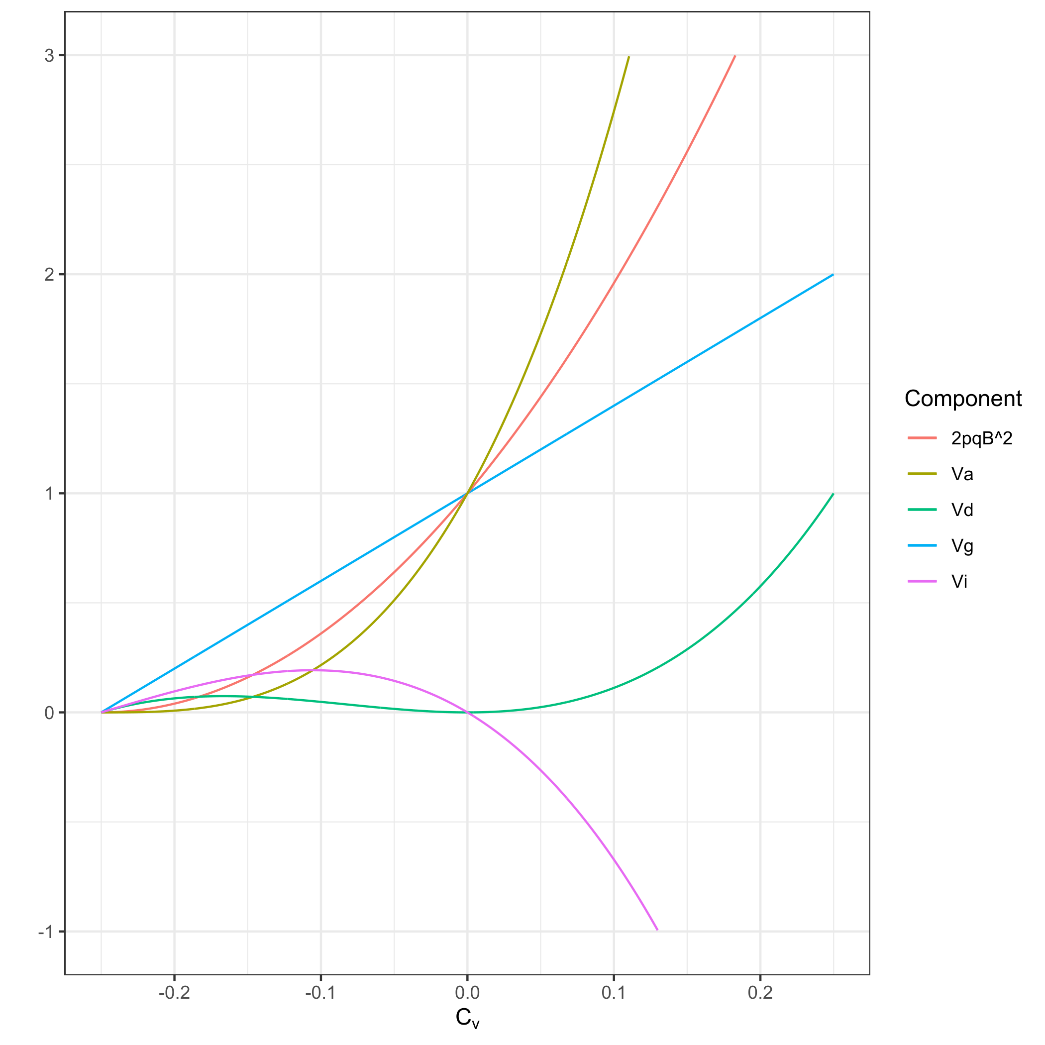
Figure 1 Within locus variance components. Variance components are represented as the ratio of their values in the real population with non-zero covariance in allelic state to their values in an idealized population in HWE, except Vd and VIad which are their values in the real population as they would be 0 in the idealized population.

3. Results and Discussion

We will now demonstrate that ancestry can cause correlations in allelic state within a locus that are identified as departures from HWE, as well as correlations in allelic state between loci that are identified as apparent linkage disequilibrium. We additionally show that within-locus correlations in allelic state in a collection of individuals in HWE are a measure of relatedness.

3.1 Ancestry affects the correlation in state within a locus

Imagine a collection of individuals who differ in their ancestry. We can think of this collection as a population, but we do not mean to assert anything in particular about breeding within this collection. Pick an individual ii at random from this collection. Individual ii has two alleles at our diploid locus vv. Call those alleles AviA_{v_i} and Avi*A^*_{v_i}. Let qviq_{v_i} be the frequency of the Av1A_{v_1} allele among individual ii's ancestors. Let CviC_{v_i} be the covariance in allelic state for our chosen individual ii. Consider CvC_v to be the covariance in allelic state in the entire collection of individuals from whom we picked individual ii. To find this, we randomize over the choice of individual ii and use the law of total covariance in equation . In this collection of individuals,

Cv=Cov[IAv,IAv*]
=E[Cov[IAv,IAv*|i]]+Cov[E[IAv|i],E[IAv*|i]]
=E[Cvi]+Cov[qvi,qvi]
=E[Cvi]+Var[qvi].

Thus, in this collection of individuals, the covariance in allelic state is the average covariance in allelic state within individuals, plus the variance in allele frequency across the ancestries of the individuals in the collection. Notice that we now think of qviq_{v_i} as the frequency of the Av1A_{v_1} allele in the ancestors of ii, a personalized allele frequency for individual ii, if you will [13], and we can sensibly discuss Var[qvi\mathrm{Var}[q_{v_i}] as the variation in this personalized frequency across individuals. Similarly we think of CviC_{v_i} as a property of ii's immediate ancestry. Are the parents of ii related to one another? Is there some form of assortative mating occurring between ii's parents? Any sort of correlation between genotype and the identity of ii's parents (inbreeding / assortative mating) will lead to E[Cvi\mathrm{E}[C_{v_i}] being non-zero. Modeling these factors' effect on phenotype might conveniently be done here. If we assume that within individuals there is no covariance in allelic state, i.e., that individuals are not inbred or the result of assortative mating, in a formal sense assuming that the two alleles are independent within an individual, then we arrive at the simplified

Cv=Var[qvi]. C_v = \mathrm{Var}[q_{v_i}].

Since variances are non-negative, we see that absent assortative mating (or some other factor that would create negative covariance in allelic state within individuals), this collection of individuals who vary in their ancestry will have a positive CvC_v, and a deficit of heterozygotes relative to HWE. This is essentially a restatement of the Wahlund effect [14], albeit without explicit reference to discrete populations. A somewhat more modern and familiar quantification of this concept is as Wright's FSTF_{ST} [15],

FST=Var[qvi]E[qvi](1E[qvi]), F_{ST} = \frac{\mathrm{Var}[q_{v_i}]}{\mathrm{E}[q_{v_i}] (1- \mathrm{E}[q_{v_i}] )} ,

where E[qvi\mathrm{E}[q_{v_i}] is the average frequency of the Av1A_{v_1} allele in the ancestors of this collection of individuals. In the Wrightian conception, we might identify E[CviE[C_{v_i}] as proportional to FISF_{IS}. There is a long history in human genetics of quantifying the variation in allele frequency across ancestry in terms of FSTF_{ST} [16-18], and it is well established that in humans, when ancestry varies across different continents, FST0.10.2F_{ST} \approx 0.1-0.2. When ancestry varies widely within a single continent, FST0.050.1F_{ST} \approx 0.05-0.1, and it tends to be less across smaller geographic regions. In the population genetics context, it is widely understood that variation in allele frequency due to ancestry leads to departures from HWE. In the quantitative genetics context, it is less widely appreciated that variation in allele frequency due to ancestry (Figure 1) can play havoc with everything, including creating dominance variance and making the additive variance larger than the total genetic variance, because negative covariance is created between the additive and dominance contributions. This is the first, albeit minor, reason all quantities in human genetics should be estimated with some procedure (linear mixed model / inclusion of PCs as covariates, etc.) that attempts to condition on the ancestry of the studied individuals. Variation in allele frequency within a single locus does not, though, create "false positive" association. From equation above, we have β=β̃(1+FST)\beta = \tilde{\beta}( 1 + F_{ST}). If we interpret effects in the Kempthorne sense, we would say the effect size differs between a population in HWE versus one out of it. In the Falconer sense, where we might think of β̃\tilde{\beta} as the "true" β\beta, we would say that departures from HWE inflate our estimate of β̃\tilde{\beta}. Of course, if β̃\tilde{\beta} is zero, this has no effect on association test statistics. However, variation in ancestry has effects on estimates of β\beta that go far beyond those of departures from HWE.

3.2 Ancestry affects the correlation in state between loci

All effect sizes in human genetics should be estimated via a method that accounts for individuals' ancestry - because variation in ancestry creates correlation in state between every site in the genome. This correlation in state between loci caused by variation in ancestry among study participants causes substantial false positive association in genetic association studies if uncorrected. To understand why this is, consider two diploid loci, vv and ww. Let IAv\mathrm{I}_{A_v} and IAw\mathrm{I}_{A_w} be the indicators that a randomly picked allele is Av1A_{v_1} and Aw1A_{w_1}, respectively. Recall [6] that the standard measures of linkage disequilibrium DD and r2r^2 can be written as

D=Cov[IAv,IAw],
r2=Cov2[IAv,IAw]Var[IAv]Var[IAw].r^2 = \frac{\mathrm{Cov}^2[\mathrm{I}_{A_v},\mathrm{I}_{A_w}]}{\mathrm{Var}[\mathrm{I}_{A_v}] \mathrm{Var}[\mathrm{I}_{A_w}]}.

Now imagine a collection of individuals whose ancestry differs from one another. Each individual ii in this collection has some ancestry where qviq_{v_i} and qwiq_{w_i} are the frequency of the Av1A_{v_1} and Aw1A_{w_1} alleles among ii's ancestors. Let DiD_i be the standard measure of linkage disequilibrium between the loci found in individual ii, a personalized linkage disequilibrium for ii.

E[IAv]=E[E[IAv|i]]
=E[qvi].
E[IAw]=E[qwi].
Var[IAv]=Var[E[IAv|i]]+E[Var[IAv|i]]
=Var[qvi]+E[qvi(1qvi)]
=Var[qvi]+E[qvi]E[qvi2]
=Var[qvi]+E[qvi](Var[qvi]+E[qvi]2)
=E[qvi](1E[qvi]).
Var[IAw]=E[qwi](1E[qwi]).
D=Cov[IAv,IAw]
=E[Cov[IAv,IAw|i]]+Cov[E[IAv|i],E[IAw|i]]
=E[Di]+Cov[qvi,qwi].
r2=(E[Di]+Cov[qvi,qwi])2E[qvi](1E[qvi])E[qwi](1E[qwi]).r^2 = \frac{(\mathrm{E}[D_i] + \mathrm{Cov}[q_{v_i},q_{w_i}] )^2}{\mathrm{E}[q_{v_i}] ( 1- \mathrm{E}[q_{v_i}] ) \mathrm{E}[q_{w_i}] ( 1- \mathrm{E}[q_{w_i}] )} .

Note that equations and follow from the law of total expectation, equation uses the definition of variance ( Var[X]=E[X2]E[X]2\mathrm{Var}[X] = \mathrm{E}[X^2] - \mathrm{E}[X]^2), and equation uses the law of total covariance. Thus, we arrive at the result that DD in the collection of individuals is the average DD within individuals, plus the covariance in allele frequencies over ancestries [19]. If loci vv and ww are not physically linked (loci on different chromosomes, say), then we expect that E[Di]=0E[D_i] = 0, and this simplifies to

D=Cov[qvi,qwi].
r2=Cov2[qvi,qwi]E[qvi](1E[qvi])E[qwi](1E[qwi]).r^2 = \frac{\mathrm{Cov}^2[q_{v_i},q_{w_i}]}{\mathrm{E}[q_{v_i}] ( 1- \mathrm{E}[q_{v_i}] ) \mathrm{E}[q_{w_i}] ( 1- \mathrm{E}[q_{w_i}] )}.

We conclude that when a group of individuals varies in ancestry, there will appear to be linkage disequilibrium (covariance in allelic state between loci) at any pair of loci that vary in frequency over ancestry, even if those loci are physically unlinked. From the fact that all correlations are bound between 1-1 and 11, we know that

Var[qv1]Var[qw1]DVar[qv1]Var[qw1].
r2=D2E[qvi](1E[qvi])E[qwi](1E[qwi])r^2 = \frac{D^2}{\mathrm{E}[q_{v_i}] ( 1- \mathrm{E}[q_{v_i}] ) \mathrm{E}[q_{w_i}] ( 1- \mathrm{E}[q_{w_i}] )}
Var[qv1]Var[qw1]E[qvi](1E[qvi])E[qwi](1E[qwi])\le \frac{\mathrm{Var}[q_{v_1}] \mathrm{Var}[q_{w_1}]}{\mathrm{E}[q_{v_i}] ( 1- \mathrm{E}[q_{v_i}] ) \mathrm{E}[q_{w_i}] ( 1- \mathrm{E}[q_{w_i}] )}
=FSTvFSTw,

where FSTvF_{{ST}_v} and FSTwF_{{ST}_w} are Wright's measures of FSTF_{ST} at locus vv and ww respectively. Thus, r2r^2 between unlinked loci is bounded by the product of FSTF_{ST} at the individual loci. If in this collection of individuals, there are only two different ancestries with any appreciable difference in allele frequency (the precise situation treated in [19]), then equality necessarily holds and D=Cov[qvi,qwi]=±Var[qvi]Var[qwi]D = Cov[q_{v_i},q_{w_i}] = \pm \sqrt{Var[q_{v_i}]Var[q_{w_i}]} regardless of the proportions of those ancestries (e.g., the respective percentages of European and African ancestry, say). To see this, call qv1,qw1q_{v_1}, q_{w_1} and qv2,qw2q_{v_2}, q_{w_2} the allele frequencies in the two different ancestries, and let c1c_1 and c2c_2, with c1=1c2c_1 = 1 - c_2, be the fraction of individuals in this collection whose ancestries are from each type. Let δqv=qv1qv2\delta_{q_v} = q_{v_1} - q_{v_2} and δqw=qw1qw2\delta_{q_w} = q_{w_1} - q_{w_2}.

Cov[qvi,qwi]=E[qviqwi]E[qvi]E[qwi]
=c1qv1qw1+c2qv2qw2(c1qv1+c2qv2)(c1qw1+c2qw2)= c_1q_{v_1}q_{w_1} + c_2q_{v_2}q_{w_2} - (c_1q_{v_1} + c_2q_{v_2})(c_1q_{w_1} + c_2q_{w_2})
=c1c2(qv1qv2)(qw1qw2)
=c1(1c1)δqvδqw.
Var[qvi]=E[qvi2]E[qvi]2
=c1qv12+c2qv22(c1qv1+c2qv2)2
=c1(1c1)δqv2.
Var[qwi]=c1(1c1)δqw2.
D=Cov[qvi,qwi]=±Var[qvi]Var[qwi].

Recall that we assumed vv and ww are independent loci (unlinked). Thus, in any collection of individuals, when there are only two ancestries significantly contributing variance in allele frequency, DD between every pair of sites in the genome will be approximately plus-or-minus the square root of the product of the variance in allele frequency at each site. These variances are defined relative to the ancestry of the individuals in the collection under consideration. Differing individuals with differing ancestry necessarily have differing variance in their allele frequency.

Human population structure can be a major cause of "false positive" association between genetic variation and phenotype whenever there is allele frequency variation in the ancestors of the individuals examined. This has been known for decades, motivating the development of a large range of complementary methods to correct for these effects (e.g., TDT, genomic control, structure, principal component analysis, linear mixed models) [20-24]. To understand more quantitatively exactly what is occurring, imagine attempting to estimate the contribution of locus vv to phenotype, and describing that effect as βv\beta_v. Let β̃v\tilde{\beta}_v be the effect of this locus if there were no variation in ancestry among the studied individuals. Thus, β̃v\tilde{\beta}_v is the effect of this locus in an idealized collection of individuals without variation in ancestry. βv\beta_v is the effect in the real collection under study (the true effect is β̃v\tilde{\beta}_v, versus the estimated effect, βv\beta_v, in the Falconer sense). Finally assume that β̃v=0\tilde{\beta}_v = 0. So, in the absence of variation in ancestry, this locus has no effect on phenotype. In the first paper in this series [6], we showed that for any pair of additive loci vv and ww, in the absence of any interactions other than correlation in allelic state

βv=β̃v+Dv,wpvqvβ̃w, \beta_v = \tilde{\beta}_v + \frac{D_{v,w}}{p_vq_v} \tilde{\beta}_w,

where Dv,wD_{v,w} is the standard linkage disequilibrium measure between loci vv and ww. Now imagine the collection of all loci wkw_k contributing an additive effect, β̃wk0\tilde{\beta}_{w_k}\ne 0, in the idealized population, but in this case we are imagining that β̃v=0\tilde{\beta}_v = 0. The total additive variance in the idealized population is

ṼA=k2pwkqwkβ̃wk2.\tilde{V}_A = \sum_k 2 p_{w_k}q_{w_k} \tilde{\beta}^2_{w_k}.

Now consider the combined effects of all loci wkw_k on βv\beta_v in a population with variation in ancestry.

βv=β̃v+kDv,wkpvqvβ̃wk\beta_v = \tilde{\beta}_v + \sum_k \frac{D_{v,w_k}}{p_vq_v} \tilde{\beta}_{w_k}
=kDv,wkpvqvβ̃wk.= \sum_k \frac{D_{v,w_k}}{p_vq_v} \tilde{\beta}_{w_k} .
βv2=(kCov[qv,qwk]pvqvβ̃wk)2\beta^2_v = \left( \sum_k \frac{\mathrm{Cov}[q_v,q_{w_k}]}{p_vq_v} \tilde{\beta}_{w_k} \right)^2
1pv2qv2(k±β̃wkVar[qv]Var[qwk])2,\approx \frac{1}{p^2_vq^2_v} \left( \sum_k \pm \tilde{\beta}_{w_k}\sqrt{\mathrm{Var}[q_{v}] \mathrm{Var}[q_{w_k}]} \right)^2,

when only a small number of ancestries contribute significantly to variation in allele frequency. This value is necessarily bigger than zero, if there is any variation in qvq_v over ancestries. Recall that a natural method to test for association between locus vv and phenotype would be to asses a null model where 2Npvqvβv22Np_vq_v\beta_v^2 is approximately χ12\chi^2_1 distributed, where NN is the number of individuals studied [25].

We thus arrive at the full intuition for the need to account for ancestry in human genetic studies. A naive χ2\chi^2 test for association between locus vv and phenotype will not have an expectation centered at 11, as the test assumes, but instead centered around a larger value that is a complex function of the covariance in allele frequencies and VAV_A. This inflation will occur at every site in the genome whose allele frequency varies over ancestry, i.e., potentially every site tested. While nearly all human geneticists understand that tests for association must account for ancestry, the reason for this is often only incompletely understood. Many discussions of this revolve around the idea that the mean phenotype (or disease prevalence for dichotomous traits) may differ between ancestries, and this difference in means causes correlation between ancestry and phenotype. Other discussions might suggest a "mechanism" for a correlation between phenotype and ancestry involving differing environmental states across ancestries, perhaps differing diets, rates of smoking, or other social determinants of health. While correlations between genes and mean phenotype or between genetic and environmental state can cause inflation of test statistics, they are in no sense required for the inflation to be pronounced. If there is additive variance for the trait, and if any of the alleles contributing to that variance differ in frequency among the ancestors of the study participants, then there will be test statistic inflation, and that inflation will increase with increasing sample size, NN, and with increasing variance in allele frequency among the participants, FSTF_{ST}. When effects are defined as the expectation of phenotype given the context in which they occur (i.e., in a Kempthorne-inspired presentation), this is not "inflation" per se, but real association between marker and phenotype, though the cause of the association is not the direct effects of the tested marker. Instead, the detected association is caused by the correlation in state between the tested marker and other variants scattered throughout the genome, i.e., the association is positive indication of the interaction—the correlation in state—between this marker and other unlinked sites. Given that the goal of association studies often is to identify loci that putatively have causal influence on phenotype, this phenomenon of association caused by interactions due to correlation in allelic state is nearly universally referred to as an issue of test statistic inflation, not one of "true" interaction, and we shall do the same.

Patterns common in disease genetics and human demographic history accentuate this inflation. The key aspect to consider is the sign of Cov[qv,qwk]βwk\mathrm{Cov}[q_v,q_{w_k}] \beta_{w_k}. Since the signs of both Cov[qv,qwk\mathrm{Cov}[q_v,q_{w_k}] and βwk\beta_{w_k} could be positive or negative, one might naively assume (hope) that the terms in the sum above will alternate signs sufficiently frequently that the mean over all SNPs might approach 00. This is unlikely to be true for disease traits. Recall we have oriented β\beta so that it is the effect of substituting the rarer allele for the more common allele. If β>0\beta > 0 then the rare allele makes the trait bigger, or in the case of a disease trait, increases the risk of disease relative to the common allele. For non-disease phenotypes there may be little reason to doubt that the sign of β\beta is "random". However, for disease traits there is good reason to believe that on average β\beta will be positive [13], because selection is likely to keep alleles rare if they increase the risk of a disease. This is especially likely if the allele has a strong effect on disease. Human demographic history suggests that Cov[qv,qwk\mathrm{Cov}[q_v,q_{w_k}] will also be positive most of the time. In general, a positive covariance between two variables implies that larger values at both variables occur more often than expected by chance. In this context it means the ancestry with the higher minor allele frequency at one locus tends to have the higher minor allele frequency at the other. In the second paper in this series [13], we saw that human demographic history tends to cause this exact pattern of correlation (conditional on alleles being present in two ancestries, one ancestry has systematically higher minor allele frequencies than the other). In that paper, the correlation in minor allele frequencies across unlinked sites appears to be the likely explanation for the most perplexing observations when applying polygenic risk scores across populations with differing ancestry. Here, the correlation in minor allele frequency induced by human demographic history is seen as the primary driver of test statistic inflation.

In this context, we can best understand how and why various procedures designed to account for this inflation work. Perhaps the most intuitively simple, but complex algorithmically, is the STRUCTURE / STRAT approach developed by Jonathan Pritchard and colleagues [22,26]. The idea is simple, variation in ancestry creates deviations from HWE within loci as well as correlation in allele frequency between loci, therefore, in principle, one can infer ancestral groups from the data [22] and then conditional on the inferred ancestry, perform association studies within ancestry groups in HWE [26]. In the structured association approach developed by Pritchard and colleagues, individuals are assigned to a subpopulation (possibly accounting for admixture with fractional cluster membership) using a model-based clustering program (STRUCTURE) [22] and association statistics are computed stratifying by subpopulation (STRAT) [26]. The approach is natural, but extremely computationally challenging for large sample sizes, and a bit sensitive to a correct a priori determination of the number of "meaningful" ancestral groups contributing to the collection.

At the other end of the computational spectrum is genomic control, pioneered by Devlin and Roeder [20]. Here the approach is incredibly simple, calculate the mean (median) χ2\chi^2 test statistic, usually called λ\lambda, from a genome-wide study and divide each site's χ2\chi^2 by λ\lambda. The intuition comes from the fact that the number of SNPs contributing to additive variance is likely very large. If so, it is not unreasonable to believe that some sort of strong law of large numbers holds, and the distribution across SNPs of βv\beta_v may therefore approximate a normal distribution, and the association test statistic will approach a non-central χ2\chi^2 with λE[βv2\lambda \sim \mathrm{E}[\beta^2_v]. That genomic control robustly controls for type-1 error in genetic studies in virtually all cases [27-28] is strong evidence in support of this intuition. While undoubtedly a robust tool, genomic control is also thought to be something of a blunt instrument, destroying "signal" in the process of achieving well calibrated type-1 error rates. By ignoring the magnitude of Cov[qv,qwk\mathrm{Cov}[q_v,q_{w_k}] and correcting for mean behavior alone, this technique penalizes all sites equally, even when an individual site vv has little or no allelic covariance with any other site in the genome, perhaps because vv has no substantial variation in allele frequency across ancestries.

Since the fundamental problem being solved is caused by covariance in allele frequency and additive variance for the trait, the most natural solution to this problem is to include both in a linear mixed model [24]. Here, the tested model takes the form

P=Svβ̃v+𝐑VA+ϵ, \vec{P} = \vec{S_v}\tilde{\beta}_v + \mathbf{R}V_A + \epsilon,

where P\vec{P} is the vector of phenotypes, Sv\vec{S_v} is a vector of minor allele counts at locus vv, 𝐑\mathbf{R} is a matrix describing the covariance in allelic state between each pair of individuals (much more on this in ), and VAV_A is the total additive variance. If both PP and SvS_v have been normalized to have mean 00, to the extent that 𝐑\mathbf{R} fully captures the covariance in allelic state between each pair of individuals and no other interactions exist, this should produce an estimate of β̃v\tilde{\beta}_v, the effect of substituting the rare allele for the common allele in a collection of individuals without ancestral variation in allele frequency - the correct β\beta in the Falconer sense, not inflated by population structure.

Linear mixed models can be quite computationally burdensome when compared to a linear model, particularly with thousands of individuals. Note that to perform certain statistical analyses within a linear mixed model framework, such as calculating individual genetic effects, the inverse of the genetic relatedness matrix 𝐑\mathbf{R} is needed. Calculating the inverse of a large relatedness matrix can be computationally demanding, especially with large sample sizes. To dramatically reduce this burden, many newer linear mixed model approaches (e.g., [29-30]) for large datasets implement algorithms that approximate the degree of relatedness among individuals in the sample without requiring a pre-computed genetic relationship matrix i.e., without explicitly calculating the covariance in allelic state between each pair of individuals. For example, a linear mixed model can be approximated with a linear model by replacing the 𝐑\mathbf{R} matrix with a subset of its eigenvectors. In this way, we can view a linear model with inclusion of principle components (PCs) derived from 𝐑\mathbf{R} [21] as a natural approximation to the more computationally burdensome linear mixed model. These approximate approaches to linear mixed models may have comparable computational efficiency to that of a linear model.

Of course, to a geneticist, the most natural way to remove the effects of variation in allele frequency over ancestries is to ensure that the test for association being performed is not affected by correlation in allelic state at unlinked markers. This can this be achieved by focusing only on alleles transmitted from parents known to be heterozygotes [23]. The transmission-disequilibrium test (TDT) counts the number of transmissions from parents known to be heterozygotes to children with some given phenotype, generally a disease state. Because Mendelian segregation is strongly regulated during meiosis to have nearly 50-50 transmission rates, regardless of the identity of any particular allele at a given site, the observed transmission rate from heterozygous parents is a function of the penetrance of the allele for the conditioned phenotype, and this transmission rate is fundamentally independent of any correlations in state at other unlinked sites [31-32]. While this approach is virtually guaranteed to solve issues associated with ancestry, it is often far harder to collect sample sets that include both parents and offspring, and undetected genotyping error can have particularly challenging effects. Computation of the TDT statistic on trios in which one parent is missing marker genotype data increases the type-1 error rate of the statistic [33] as does genotyping error, which can cause apparent over-transmission of common alleles [34-35].

3.3 Phenotypic covariance, relatedness, and the covariance in allelic state

The first paper in this series [6] derived the covariance between individuals in a generalized form. Here we focus on a very specialized case where there is potentially correlation in genotypic state, but no other non-additive interactions of any kind - no dominance, additivity between all loci, and no correlation in state of non-genetic factors. Imagine a collection of individuals that might be a single population in HWE or could be collection of individuals with differing and complex ancestry. We are interested in two randomly picked individuals from this collection; call them individuals 11 and 22 and their phenotypes P1P_1 and P2P_2. At some locus vv contributing to this phenotype, let Sv1S_{v_1} and Sv2S_{v_2} be the counts of minor alleles, Av1A_{v_1}, in individual 11 and 22, respectively. Let S1\vec{S_1} and S2\vec{S_2} be the vector of these counts over all loci contributing to the phenotype. Let αv01\alpha_{v_{0_1}} and αv02\alpha_{v_{0_2}} be the average phenotype of an individual with the common allele at locus vv in individuals with ancestral minor allele frequencies qv1q_{v_1} and qv2q_{v_2} respectively. While the allelic effect α\alpha will be a function of allele frequency, assume the difference in allelic effects β̃=α1α0\tilde{\beta} = \alpha_1 - \alpha_0 [13] is the same in all individuals regardless of allele frequency.

E[P1|S1]=v(β̃vSv1+2αv01).
E[P2|S2]=v(β̃vSv2+2αv02).
E[P1P2|S1,S2]=(v(β̃vSv1+2αv0))(v(β̃vSv2+2αv0)).
Cov[P1,P2|S1,S2]=E[P1P2|S1,S2]E[P1|S1,S2]E[P2|S1,S2]
=0.
Cov[P1,P2]=Cov[E[P1|S1,S2],E[P2|S1,S2]]
+E[Cov[P1,P2|S1,S2]]
=Cov[v(β̃vSv1+2αv01),v(β̃vSv2+2αv02)]
=vβ̃v2Cov[Sv1,Sv2]+vwβ̃vβ̃wCov[Sv1,Sw2].

Line 77 uses the lack of dominance or any other interactions extensively. Thus, for an additive trait, the covariance between individuals is the sum over all contributing loci of β̃2\tilde{\beta}^2 multiplied by the covariance in minor allele counts, plus the sum of the product of two different β\beta's, and their covariance in allelic state (LD) for pairs of sites across the genome.

3.3.1 Relatedness for single population in Hardy-Weinberg equilibrium

If individuals 11 and 22 were drawn from a single population where all loci are unlinked and in HWE, then the second sum in is 00. In a single population, if individuals 11 and 22 share fraction rr of the their genome identical-by-descent (IBD) because they share recent common ancestors, and if r0,r1r_0, r_1, and r2r_2 are the fraction of the genome where exactly 0,10,1 and 22 alleles are shared IBD, then we arrive at the the familiar

E[Sv1]=E[Sv2]=2qv.
Cov[Sv1,Sv2]=i=0,1,2E[Sv1Sv2|ri]4qv2
=r0(4qv2)+r1(qv(4qv2+4pvqv+pv2)+pvqv2)
+r2(4qv2+2pvqv)4qv2
=r1(pv2qv+pvqv2)+2r2pvqv
=pvqv(r1+2r2)
=2pvqvr.
r=Cov[Sv1,Sv2]2pvqv.r = \frac{\mathrm{Cov}[ S_{v_1}, S_{v_2}]}{2p_vq_v}.

The covariance in genotypic state at a locus between two individuals is the relatedness between the individuals multiplied by 2pq2pq, for a collection of individuals in HWE. In this fashion we now see that rr called relatedness is also by definition rr, the correlation in genotypic state, for a collection of individuals in HWE. Quite literally, relatedness is the correlation in genotypic state. Because of this, for any pair of individuals, we can imagine using the observed correlation in genotypic state across a collection of loci to estimate the relatedness of those two individuals. For instance, in a collection of NN distinct SNPs vv in HWE, we could estimate the relatedness rijr_{ij} between a randomly picked pair of individuals ii and jj as

r̂ij=1NvCov[Svi,Svj]2pvqv\hat{r}_{ij} = \frac{1}{N} \sum_v \frac{\mathrm{Cov}[ S_{v_i}, S_{v_j}]}{2p_vq_v}
=1Nv(Svi2qv)(Svj2qv)2pvqv.= \frac{1}{N} \sum_v\frac{(S_{v_i}-2q_v)(S_{v_j}-2q_v)}{2p_vq_v} .

Thus, if we had a random collection of individuals drawn from a single population in HWE and had a collection of SNP genotypes in those individuals, we could estimate the relatedness between each pair of individuals directly from the genotypes. A matrix 𝐑\mathbf{R} whose elements rijr_{ij} are calculated as above is an estimate of the relatedness of those individuals over the SNPs used in the estimate. Of course, if the collection of individuals or SNPs used in the estimate is biased, it is possible the estimate of relatedness might also be biased in some fashion. Nevertheless, this method of estimation should be fundamentally robust with a sufficiently large number of SNPs in any collection of individuals in HWE.

3.3.2 Phenotypic covariance in the presence of population structure

In a collection of individuals with complex ancestries, we again think of an individual's ancestry as determining their personal allele frequency, qviq_{v_i}, at locus vv. We further imagine individuals who do not share an ancestry are not closely related to one another so that rij=0r_{ij} = 0. Thus, when individual ii and jj are related at locus vv, qvi=qvjq_{v_i} = q_{v_j}. Let IqvijI_{q_{v_{ij}}} be the indicator that individuals ii and jj share an ancestry at locus vv so that they have equal personalized allele frequencies at locus vv, qvi=qvjq_{v_i} = q_{v_j}. E[Iqvij\mathrm{E}[I_{q_{v_{ij}}}] is the probability these two individuals have the same ancestry at this site. Letting qv\bar{q}_v and Var[qv\mathrm{Var}[q_v] be the overall mean and variance in allele frequency across all individuals in the collection,

Cov[Svi,Svj]=Cov[E[Svi|Iqvij],E[Svj|Iqvij]]
+E[Cov[Svi,Svj|Iqvij]].
Cov[E[Svi|Iqvij],E[Svj|Iqvij]]=Cov[2qvi,2qvj]
=4Cov[qvi,qvj]
=4(Cov[E[qvi|Iqvij],E[qvj|Iqvij]]
+E[Cov[qvi,qvj|Iqvij]])
=4E[Iqvij]Var[qv].
E[Cov[Svi,Svj|Iqvij]]=E[Iqvij(2pviqvirij)
+(1Iqij)Cov[Svi,Svj|Iqvij=0]]
=E[Iqvij]2qvpvrij.
Cov[Svi,Svj]=E[Iqvij](rij(2qvpv)+4Var[qv])
=E[Iqvij]2qvpv(rij+2FSTv).

Returning attention to the second sum in 80, begin by writing SviS_{v_i} as the sum of two different indicators ( IAviI_{A_{v_i}} + IAvi*I_{A^*_{v_i}}) that individual ii has the Av1A_{v_1} allele

Svi=IAvi+IAvi*.
Swj=IAwj+IAwj*.
Cov[Svi,Swj]=Cov[IAvi+IAvi*,IAwj+IAwj*]
=4Cov[IAvi,IAwj]
=4(E[Cov[IAvi,IAwj|Iqvij,Iqwij]
+Cov[E[IAvi|Iqvij,Iqwij],E[IAwj|Iqvij,Iqwij]].

To finish we need to add the insight that when two individuals are picked at random, if they share no ancestry at a given locus, the allele draws are independent and there is no covariance in state between different loci, so that

E[Cov[IAvi,IAwj|Iqvij,Iqwij]=E[IqvijIqwijCov[qv,qw]]
=E[IqvijIqwij]Cov[qvi,qwi]
=E[IqvijIqwij]Dv,w.
Cov[E[IAvi|Iqvij,Iqwij],E[IAwj|Iqvij,Iqwij]]=0.

Putting this all together with the assumption that local ancestry does not differ significantly across the genome, in other words that for all choices of vv and ww, E[Iqvij]E[Iqwij]=Mij\mathrm{E}[ I_{q_{v_{ij}}}] \approx \mathrm{E}[ I_{q_{w_{ij}}}] = M_{ij}, then

Cov[Pi,Pj]=vE[Iqvij]2pvqvβ̃v2(rij+2FSTv)
+vw4β̃vβ̃wE[IqvijIqwij]Dv,w
=vMijṼav(rij+2FSTv)+vw4β̃vβ̃wMij2Dv,w.

Recall that β̃v\tilde{\beta}_v is the effect of this locus in an idealized collection of individuals without variation in ancestry (i.e., Cv=0C_v = 0, in HWE). As such, Ṽav=2pvqvβ̃v2\tilde{V}_{a_v} = 2 \bar{p}_v \bar{q}_v \tilde{\beta}_v^2 is the additive variance due to this locus and ṼA=vṼav\tilde{V}_A = \sum_v\tilde{V}_{a_v} is the total additive variance in the idealized population. If the collection of individuals is an approximately equal mixture of two major ancestry groups, so every individual shares approximately half of their ancestry with every other individual such that Mij0.5M_{ij} \approx 0.5, an almost natural looking result appears

Cov[Pi,Pj]vṼav(rij2+FSTv)+vwβ̃vβ̃wDv,w\mathrm{Cov}[P_i,P_j] \approx \sum_v \tilde{V}_{a_v} \left(\frac{r_{ij}}{2} + F_{ST_v}\right) + \sum_{v \ne w} \tilde{\beta}_v\tilde{\beta}_w D_{v,w}
ṼA(rij2+FST)+vwβ̃vβ̃wDv,w,\approx \tilde{V}_A \left(\frac{r_{ij}}{2} + F_{ST}\right) + \sum_{v \ne w} \tilde{\beta}_v\tilde{\beta}_w D_{v,w},

where rijr_{ij} is the relatedness between individuals ii and jj and FSTF_{ST} is something like the average FSTF_{ST} across all loci contributing to the phenotype. Of course, as shown above Dv,wD_{v,w} is a function of the variation in allele frequency across the ancestries of the individuals in the collection.

Covariance in genotypic state can therefore be described in several ways. It is relatedness in a collection in HWE. It is also the standard measure of linkage disequilibrium, and variation in ancestry induces LD between sites. Finally it can be the primary "cause" of inflation of test statistics in genetic association studies. Overall, the resemblance between individuals with complex ancestry is a function of VAV_A, relatedness among those individuals, and the variation in allele frequency over ancestries.

4. Conclusions

In the two papers that comprise the third part of this series, we distinguish interactions arising from correlations in state between factors from those arising from non-additivity of independent factors.

Correlation in state of factors occurs commonly. Here we understand departures from HWE as a form of interaction caused by correlation in allelic state within a genotype, which can result from variation in allele frequency across ancestry. Correlation in state within loci has very complex impacts, and can cause changes in effects (changes in means) as well as increases or decreases in the total variance relative to the sum of the individual factor variances. In the presence of correlation in state, concepts such as dominance variance or interaction variance are often not well defined, and may appear to be negative, because non-independence of the state of factors can create negative covariance. In the presence of correlations in allelic state, a locus that would have been completely additive had it been in HWE has both additive and dominance variance; its total genetic variance is no longer the sum of the additive and dominance variance; the additive variance is no longer the same as 2pqβ22pq\beta^2, and heritability is now a function of the correlation in allelic state in each relative (which could differ between them). Correlations in allelic and genotypic state dramatically alter our intuitions and our quantitative genetic estimates, and thus should be accounted for explicitly.

Variation in ancestry can create correlation in state between every site in the genome. Whenever there is ancestry variation in a collection of examined individuals, any pair of loci that vary in frequency over ancestry will appear to be in linkage disequilibrium, even if those loci are physically unlinked. If there is additive variance for the trait, and if any of the alleles contributing to that variance differ in frequency among the ancestors of the study participants, then there will be test statistic inflation for any naive test correlating allele frequency with phenotype. Correlation in minor allele frequency induced by human demographic history is the primary driver of this inflation in association studies, and we reviewed several approaches to account for this inflation [20,22-24,26].

Correlation is genotypic state between two individuals is also a measure of the relatedness of those individuals. Departures from Hardy-Weinberg Equilibrium (HWE), linkage disequilibrium (LD), population structure, and relatedness are generally viewed by population geneticists as distinct concepts. However, as we have shown, departures from HWE, LD, and relatedness are all measures of the correlation in genotypic state among the individuals in a collection. While it is often useful to treat the effects of each of these independently of one another, all of them can be understood as forms of genetic interaction caused by correlation in state—between alleles within a locus, between pairs of sites across the genome, and between individuals.

Declarations

Ethics Statement

Not applicable.

Consent for Publication

Not applicable.

Availability of Data and Material

Not applicable.

Funding

This study was supported by NIH Grants RF1 AG071170 and U01 DK134191.

Competing Interests

David J. Cutler is a member of the Editorial Board of the journalHuman Population Genetics and Genomics. The author was not involved in the journal’s review of or decisions related to this manuscript. The authors have declared that no other competing interests exist.

Author Contributions

All authors participated in the derivation, writing, and editing of this work.

Acknowledgement

This work has benefited from many helpful suggestions by Greg Gibson, and long conversations with Loic Yengo.

References

1. de Leeuw CA, Mooij JM, Heskes T, Posthuma D. MAGMA: generalized gene-set analysis of GWAS data. PLoS Comput Biol. 2015;11(4):e1004219. [Google Scholar] [CrossRef]
2. He X, Sanders SJ, Liu L, De Rubeis S, Lim ET, Sutcliffe JS. Integrated model of de novo and inherited genetic variants yields greater power to identify risk genes. PLoS Genet. 2013;9(8):e1003671. [Google Scholar] [CrossRef]
3. Wu MC, Lee S, Cai T, Li Y, Boehnke M, Lin X. Rare-variant association testing for sequencing data with the sequence kernel association test. Am J Hum Genet. 2011;89(1):82-93. [Google Scholar] [CrossRef]
4. Zhan X, Hu Y, Li B, Abecasis GR, Liu DJ. RVTESTS: an efficient and comprehensive tool for rare variant association analysis using sequence data. Bioinformatics. 2016;32(9):1423-1426. [Google Scholar] [CrossRef]
5. Jodeiry K, Bass AJ, Epstein MP, Cutler DJ. The Quantitative Genetics of Human Disease: 3b Interactions - Non-Additivity and Missing Heritability. Hum Popul Genet Genom. 2025. [Google Scholar]
6. Cutler D, Jodeiry K, Bass A, Epstein M. The quantitative genetics of human disease: 1. Foundations. 2023;3(4):0007. [Google Scholar] [CrossRef]
7. Kempthorne O. The Theoretical Values of Correlations between Relatives in Random Mating Populations. Genetics. 1955;40(2):153-167. [Google Scholar] [CrossRef]
8. Fisher RA. The Correlation between Relatives on the Supposition of Mendelian Inheritance. Trans R Soc Edinburgh. 1918;52:399. [Google Scholar]
9. Kempthorne O. The Correlation between Relatives in a Simple Autotetraploid Population. Genetics. 1955;40(2):168-174. [Google Scholar] [CrossRef]
10. Horner TW, Kempthorne O. The Components of Variance and the Correlations between Relatives in Symmetrical Random Mating Populations. Genetics. 1955;40(3):310-320. [Google Scholar] [CrossRef]
11. Kempthorne O. The Correlations between Relatives in Inbred Populations. Genetics. 1955;40(5):681-691. [Google Scholar] [CrossRef]
12. Population Genetics : A Concise Guide. 2nd ed. 2004. [Google Scholar]
13. Cutler D, Jodeiry K, Bass A, Epstein M. The Quantitative Genetics of Human Disease: 2 Polygenic Risk Scores. Hum Popul Genet Genom 2024;4(3):0008. 2024;4(3):0008. [Google Scholar] [CrossRef]
14. Wahlund S. ZUSAMMENSETZUNG VON POPULATIONEN UND KORRELATIONSERSCHEINUNGEN VOM STANDPUNKT DER VERERBUNGSLEHRE AUS BETRACHTET. Heredity (Edinb). 1928;11(1):65-106. [Google Scholar] [CrossRef]
15. WRIGHT S. Genetical structure of populations. Nature. 1950;166(4215):247-249. [Google Scholar] [CrossRef]
16. Lewontin RC. The Apportionment of Human Diversity. In: Dobzhansky T, Hecht MK, Steere WC, editors. 1972. [Google Scholar] [CrossRef]
17. Roychoudhury AK, Nei M. Human polymorphic genes: world distribution. New York: Oxford University Press. 1988. [Google Scholar]
18. Jakobsson M, Scholz SW, Scheet P, Gibbs JR, VanLiere JM, Fung HC. Genotype, haplotype and copy-number variation in worldwide human populations. Nature. 2008;451(7181):998-1003. [Google Scholar] [CrossRef]
19. Nei M, Li WH. Linkage disequilibrium in subdivided populations. Genetics. 1973;75(1):213-219. [Google Scholar] [CrossRef]
20. Devlin B, Roeder K. Genomic control for association studies. Biometrics. 1999;55(4):997-1004. [Google Scholar] [CrossRef]
21. Price AL, Patterson NJ, Plenge RM, Weinblatt ME, Shadick NA, Reich D. Principal components analysis corrects for stratification in genome-wide association studies. Nat Genet. 2006;38(8):904-909. [Google Scholar] [CrossRef]
22. Pritchard JK, Stephens M, Donnelly P. Inference of population structure using multilocus genotype data. Genetics. 2000;155(2):945-959. [Google Scholar] [CrossRef]
23. Spielman RS, McGinnis RE, Ewens WJ. Transmission test for linkage disequilibrium: the insulin gene region and insulin-dependent diabetes mellitus (IDDM). Am J Hum Genet. 1993;52(3):506-516. [Google Scholar]
24. Zhu X, Zhang S, Zhao H, Cooper RS. Association mapping, using a mixture model for complex traits. Genet Epidemiol. 2002;23(2):181-196. [Google Scholar] [CrossRef]
25. Bulik-Sullivan BK, Loh PR, Finucane HK, Ripke S, Yang J; Schizophrenia Working Group of the Psychiatric Genomics Consortium; et al. LD Score regression distinguishes confounding from polygenicity in genome-wide association studies. Nat Genet. 2015;47(3):291-295. [Google Scholar] [CrossRef]
26. Pritchard JK, Stephens M, Rosenberg NA, Donnelly P. Association mapping in structured populations. Am J Hum Genet. 2000;67(1):170-181. [Google Scholar] [CrossRef]
27. Hao K, Li C, Rosenow C, Wong WH. Detect and adjust for population stratification in population-based association study using genomic control markers: an application of Affymetrix Genechip Human Mapping 10K array. Eur J Hum Genet. 2004;12(12):1001-1006. [Google Scholar] [CrossRef]
28. Yang J, Weedon MN, Purcell S, Lettre G, Estrada K, Willer CJ. Genomic inflation factors under polygenic inheritance. Eur J Hum Genet. 2011;19(7):807-812. [Google Scholar] [CrossRef]
29. Loh PR, Tucker G, Bulik-Sullivan BK, Vilhjálmsson BJ, Finucane HK, Salem RM. Efficient Bayesian mixed-model analysis increases association power in large cohorts. Nat Genet. 2015;47(3):284-290. [Google Scholar] [CrossRef]
30. Zhou W, Nielsen JB, Fritsche LG, Dey R, Gabrielsen ME, Wolford BN. Efficiently controlling for case-control imbalance and sample relatedness in large-scale genetic association studies. Nat Genet. 2018;50(9):1335-1341. [Google Scholar] [CrossRef]
31. Ewens WJ, Spielman RS. The transmission/disequilibrium test: history, subdivision, and admixture. Am J Hum Genet. 1995;57(2):455-464. [Google Scholar]
32. Spielman RS, Ewens WJ. The TDT and other family-based tests for linkage disequilibrium and association. Am J Hum Genet. 1996;59(5):983-989. [Google Scholar]
33. Curtis D, Sham PC. A note on the application of the transmission disequilibrium test when a parent is missing. Am J Hum Genet. 1995;56(3):811-812. [Google Scholar]
34. Gordon D, Heath SC, Liu X, Ott J. A transmission/disequilibrium test that allows for genotyping errors in the analysis of single-nucleotide polymorphism data. Am J Hum Genet. 2001;69(2):371-880. [Google Scholar] [CrossRef]
35. Mitchell AA, Cutler DJ, Chakravarti A. Undetected genotyping errors cause apparent overtransmission of common alleles in the transmission/disequilibrium test. Am J Hum Genet. 2003;72(3):598-610. [Google Scholar] [CrossRef]
Download PDF

Share this article

About Us Journals Join Us Submit Fees Contact