The Quantitative Genetics of Human Disease: 3B Interactions—Non-Additivity and Missing Heritability

Sections

Abstract
1. Introduction
2. Materials and Methods
3. Results and Discussion
4. Conclusions
Declarations
Reference

Human Population Genetics and Genomics 2025;5(4):0009 | https://doi.org/10.47248/hpgg2505040009

Original Research Open Access

The Quantitative Genetics of Human Disease: 3B Interactions—Non-Additivity and Missing Heritability

Kiana Jodeiry ^1,2 , Andrew J. Bass ^2,3,† , Michael P. Epstein ^2,3 , David J. Cutler ^2,3

1. Department of Psychology, Emory University, Atlanta, Georgia 30322, USA
2. Center of Computational and Quantitative Genetics, Emory University, Atlanta, Georgia 30322, USA
3. Department of Human Genetics, Emory University, Atlanta, Georgia 30322, USA

† Current address: Department of Medicine, University of Cambridge, Addenbrooke’s Hospital, Hills Road, Cambridge, UK

Correspondence: David J. Cutler

Academic Editor(s): Carina Schlebusch, Lounès Chikhi

Received: Oct 30, 2024 | Accepted: Dec 19, 2025 | Published: Dec 30, 2025

© 2025 by the author(s). This is an Open Access article distributed under the Creative Commons License Attribution 4.0 International (CC BY 4.0) license, which permits unrestricted use, distribution, and reproduction in any medium or format, provided the original work is correctly credited.

Cite this article: Jodeiry K, Bass AJ, Epstein MP, Cutler DJ. The Quantitative Genetics of Human Disease: 3B Interactions—Non-Additivity and Missing Heritability. Hum Popul Genet Genom. 2025;5(4):0009. https://doi.org/10.47248/hpgg2505040009

Abstract

The third section of an anticipated four paper series distinguishes two different forms of genetic interactions. The first paper of our discussion on genetic interactions described interactions arising from correlation between genotypic and/or environmental states. In this, the second paper, we describe interactions arising from non-additivity between uncorrelated factors (epistasis). We also discuss in detail the concept of "missing heritability.” While this phrase is sometimes used to mean what might more precisely be called "still unidentified heritable factors," this phrase also describes the observation that heritability when studied in close relatives almost always produces estimates significantly larger than when studied in distant relatives. While still unidentified heritable factors can be discovered via whole genome sequencing in ever increasing sample sizes, differing estimates of heritability from close versus distant relatives implies the existence of some form of interaction. Several types of interaction could explain this phenomenon. We conclude by focusing on a particular form of interaction that has been widely ignored, interactions caused by non-additivity arising from the cis-regulation of gene expression. By exploring varying patterns of two-locus haplotypic effects, we show that the existence of two or more variants each influencing the expression of the same gene can give rise to substantial non-additive interactions, and that those interactions can be particularly large when the variants are rare. Additive-by-additive genetic interactions induced by gene regulation have the potential to fully explain the observation of missing heritability.

Keywords

quantitative genetics, human disease, genetic interactions, missing heritability, gene regulation

1. Introduction

The phenomenon known as “missing heritability" is most simply described as estimates of heritability differ between differing techniques used to make the estimate, where estimates from close relatives are almost uniformly larger than any other technique used to make that estimate. We will argue that this pattern is an indication that some form of interaction must exist, and we pay particular attention to higher-order additive-by-additive interactions caused by non-additivity between variants involved in the regulation of the same gene’s expression.

In general, non-additivity means that the average phenotype given a combination of alleles at two or more different loci is not the sum of the average phenotypes given each allele individually. Genetic risk for complex traits will often act via proximate changes in gene expression, structure, or function (i.e., genetically regulated gene expression or protein sequence), and complex trait-associated SNPs are significantly more likely to be expression quantitative trait loci than minor allele frequency-matched SNPs [1–3]. Multiple genetic variants located in regulatory elements such as enhancers and transcription factor binding sites (e.g., eQTLs) can act in concert to modulate the transcriptional activities of target genes that are nearby in a process known as cis-regulation [4]. We demonstrate that it is the cis-regulation of gene expression by multiple loci that naturally induces higher-order additive-by-additive interactions, which could contribute a substantial fraction of the "missing heritability” of complex traits.

To a significant extent, higher-order interactions have been widely ignored in genetic studies as it has not been clear under what circumstances (what models) we should expect higher-order interactions to exist. We describe models of cis-gene regulation that predict the existence of higher-order interactions and develop analytical bounds for the possible size of those interactions as a function of single-site properties (allele frequencies and additive/main effects). We explore several relationships among two-locus haplotypic effects representing cis-regulatory network patterns that include loss of function alleles, general gene regulation models where loci can act as enhancers or repressors, and regulatory mechanisms at the level of topologically associating domains (TADs) in the context of linkage disequilibrium and without LD. For these models, we derive the maximum possible higher-order additive-by-additive interaction variance and demonstrate that additive-by-additive interaction variance has the potential to be largest when the minor alleles at the loci are rare. Our aim is to provide a coherent explanation of one of the most basic questions in human genetics today: "Why do modern SNP-based estimators of heritability suggest that additive variance is much lower than familial studies predict?”

2. Materials and Methods

We begin with a reminder [5] of our Kempthorne [6] inspired definition of "effect.” The effect of being in any particular state of some factor, or any collection of states, is defined to be the average phenotype of individuals who are in that state or collection of states. The effect of an A₁ allele is the average phenotype of individuals who possess the A₁ allele. The effect of the combination of the A₁ allele and environmental state e₁ is the average phenotype of individuals who have the combination of the A₁ allele along with environmental state e₁. An interaction is said to exist whenever the effect of a combination of states is not equal to the sum of the individual state effects. It is helpful to distinguish two forms of interaction. Interactions can arise from correlation in the state of two factors, i.e., the chance of having allele A₁ might be correlated with the chance of being in environmental state e₁ – these were discussed in the previous paper in this series [7]. Alternatively, the state of factors might be independent, but the effect of two or more factor states is different from the sum of the individual state effects: the independent factors are "non-additive" – these are the interactions discussed in this paper. Interaction due to non-additivity of independent states is often called epistasis, but this term is far from consistently applied or used. Although asserted several times previously, here we show for the first time that non-additivity of independent factors only increases total variance.

In attempt to be as general as possible, imagine two factors, call them X and Y, that contribute to phenotype. These factors might be genetic or environmental with a discrete or continuous number of different states that they can attain. Let x and y be possible states of X and Y. Let ξ_X=x be the effect of factor X being in state x, and ξ_Y=y be the effect of factor Y being in state y. Let $κ_{X_{x}, Y_{y}}$ be the combined effect of X being in state x and Y being in state k. Let $δ_{X_{x}, Y_{y}}$ be the deviation from additivity of these two factors. Finally assume the states of X and Y are independent, meaning Pr[X = x|Y = y] = Pr[X = x], and vice versa. Call the phenotype in question P, and recall that P has been normalized so that its mean is 0.

(1)

\begin{matrix} ξ_{X = x} & = & E [P | X = x] . \end{matrix}

(2)

\begin{matrix} ξ_{Y = y} & = & E [P | Y = y] . \end{matrix}

(3)

\begin{matrix} κ_{X_{x}, Y_{y}} & = & E [P | X = x, Y = y] . \end{matrix}

(4)

\begin{matrix} δ_{X_{x}, Y_{y}} & = & κ_{X_{x}, Y_{y}} - (ξ_{X = x} + ξ_{Y = y}) . \end{matrix}

(5)

\begin{matrix} κ_{X_{x}, Y_{y}} & = & ξ_{X = x} + ξ_{Y = y} + δ_{X_{x}, Y_{y}} . \end{matrix}

Associate with these effects random variables z_X, z_Y, k_X,Y, and d_X,Y = k_X,Y − (z_X + z_Y) whose values are determined by the effects of being in the states of X and Y. Thus, if factor X is in state x and factor Y is in state y, then z_X = ξ_X=x, z_Y = ξ_Y=y, k_X,Y = κX_x,Y_y, and $d_{X, Y} = δ_{X_{x}, Y_{y}}$ . Given the law of total expectation (for any random variables X and Y, E[X] = E[E[X|Y]]), all of these random variables have mean 0 because P has mean 0.

(6)

\begin{matrix} E [z_{X}] & = & E [E [P | X]] = E [P] = 0. \end{matrix}

(7)

\begin{matrix} E [z_{Y}] & = & E [E [P | Y]] = E [P] = 0. \end{matrix}

(8)

\begin{matrix} E [k_{X, Y}] & = & E [E [P | X, Y]] = E [P] = 0. \end{matrix}

(9)

\begin{matrix} E [d_{X, Y}] & = & E [k_{X, Y} - (z_{X} + z_{Y})] = 0. \end{matrix}

The key insight is that when the states of X and Y are independent, d_X,Y is orthogonal to both z_X and z_Y, and therefore the total variance (Var[k_X,Y]) will be the sum of the individual variance components (Var[k_X,Y] = Var[z_X] + Var[z_Y] + Var[d_X,Y]). To see this explicitly,

(10)

\begin{matrix} Var [k_{X, Y}] & = & E [{(k_{X, Y})}^{2}] \end{matrix}

(11)

\begin{matrix} = & E [{(z_{X} + z_{Y} + d_{X, Y})}^{2}] \end{matrix}

(12)

\begin{matrix} = & E [z_{X}^{2}] + E [z_{Y}^{2}] + E [d_{X, Y}^{2}] \end{matrix}

(13)

\begin{matrix} + 2 (E [z_{X} z_{Y}] + E [z_{X} d_{X, Y}] + E [z_{X} d_{X, Y}]) \end{matrix}

(14)

\begin{matrix} = & Var [z_{X}] + Var [z_{Y}] + Var [d_{X, Y}], \end{matrix}

because of the independence of X and Y. To better understand why this is, note that

(15)

\begin{matrix} E [z_{X} z_{Y}] & = & E [z_{X}] E [z_{Y}] = 0. \end{matrix}

(16)

\begin{matrix} E [z_{X} d_{X, Y}] & = & E [z_{X} (k_{X, Y} - (z_{X} + z_{Y}))] \end{matrix}

(17)

\begin{matrix} = & E [z_{X} k_{X, Y}] - E [z_{X}^{2}] - E [z_{X} z_{Y}] \end{matrix}

(18)

\begin{matrix} = & E [E [P | X] E [P | X, Y]] - E [z_{X}^{2}] \end{matrix}

(19)

\begin{matrix} = & E [z_{X}^{2}] - E [z_{X}^{2}] = 0. \end{matrix}

(20)

\begin{matrix} E [z_{Y} d_{X, Y}] & = & 0. \end{matrix}

Because X and Y are independent, we have swapped the orders of integration to remove Y from E[z_Xk_X,Y] and X from E[z_Yk_X,Y]. Altogether this establishes the "simple” intuition that all quantitative geneticists have and which is taught to students. When the states of factors are independent, any interaction (non-additivity) causes an increase in total variance, and that variance is quantified by Var[d_X,Y], which is the average squared deviation ( $δ_{X, Y}^{2}$ ) from additivity of these two factors X and Y.

2.1 Non-additive interactions between factors with uncorrelated states causes variance differences within the states of a factor

Focus now on factor X which can take on multiple states, x. Assume that the states of X are uncorrelated with the state of any other factor. Any non-additive interaction involving X causes differing variance in phenotype between the states of X. In general, if there are f other factors Y_k, 1 ≤ k ≤ f which interact non-additively with factor X, and y_k is a possible state for factor Y_k, then

(21)

\begin{matrix} E [P | X = x] & = & ξ_{X = x} . \end{matrix}

(22)

\begin{matrix} E [P | Y_{k} = y_{k}] & = & ξ_{Y_{k} = y_{k}} . \end{matrix}

(23)

\begin{matrix} δ_{X = x, Y_{k} = y_{k}} & = & E [P | X = x, Y_{k} = y_{k}] - (ξ_{X = x} + ξ_{Y_{k} = y_{k}}) . \end{matrix}

(24)

\begin{array}{l} δ_{X = x, Y_{k} = y_{k}, Y_{j} = y_{j}} & = & E [P | X = x, Y_{k} = y_{k}, Y_{j} = y_{j}] \\ - (ξ_{X = x} + ξ_{Y_{k} = y_{k}} + ξ_{Y_{j} = y_{j}} \\ + δ_{X = x, Y_{k} = y_{k}} + δ_{X = x, Y_{j} = y_{j}} + δ_{Y_{k} = y_{k}, Y_{j} = y_{j}}) . \end{array}

(25)

\begin{array}{l} Var [Var [P | X]] & = & \sum_{k}^{f} Var [E [d_{X, Y_{k}}^{2}] | X] \\ + \sum_{k}^{f} \sum_{j}^{f} Var [E [d_{X, Y_{k}, Y_{j}}^{2}] | X] \\ + \sum_{k}^{f} \sum_{j}^{f} \sum_{m}^{f} . .. + ..., \end{array}

where the continuing sums are for all the higher order deviations from additivity. Intuitively, this is telling us that when residual variance in phenotype differs between differing states of the same factor, then there exists interactions involving that factor. When states of factors are uncorrelated with anything else, if there is significant variation in the variance in the phenotype given the states, then this factor must interact with at least one other thing. The variance in variance in phenotype is the sum of the variances of the average squared deviations from additivity between this factor and its interacting partners. In this manner, it is possible to test for "latent” interactions by testing for differences in the residual phenotypic variance between states of a factor (see Figure 1). If the states of a factor differ in their residual phenotypic variance then that factor interacts with something. Its interacting partner may be unidentified (i.e., latent), but such a partner(s) must exist. Therefore SNPs involved in non-additive interactions can be directly discovered by examining the variance in residual phenotypic variance given the genotype. Variance-based testing procedures, which do not require the interacting variable(s) to be identified, prioritize genetic variants associated with the variance of the phenotype (vQTLs) by detecting unequal residual phenotypic variance among genotype categories at a specific SNP (i.e., heteroskedasticity) [8–10]. Genome-wide screening procedures that identify a reduced set of variants with potential interaction effects can circumvent some of the challenges inherent in attempting to find interactions among tens of millions of factors [11].

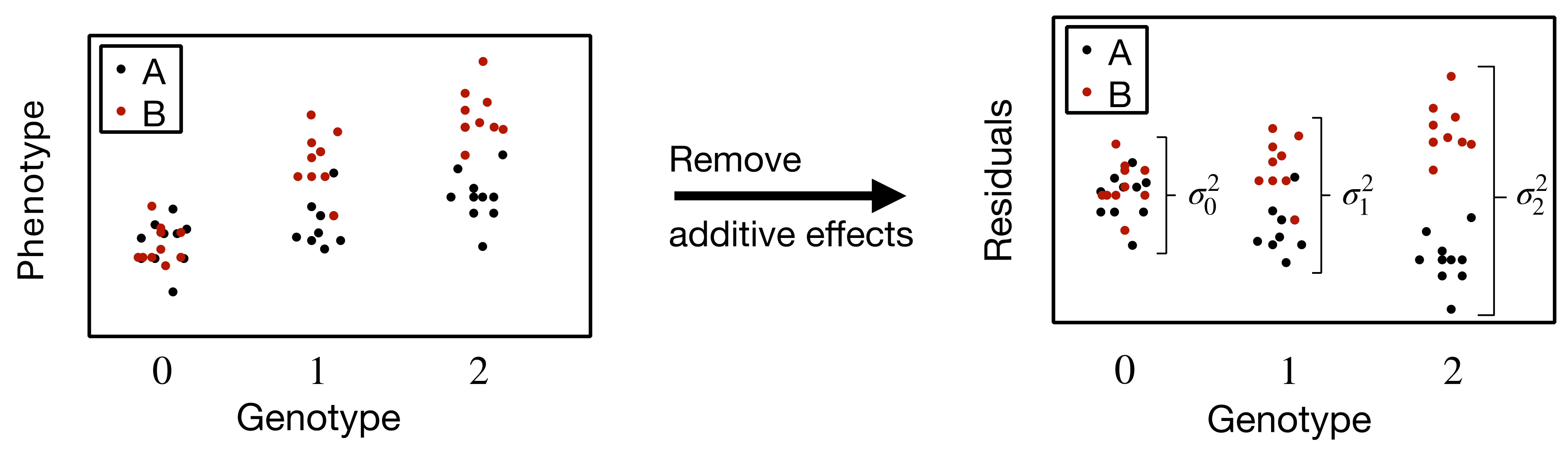
Figure 1 Differing residual phenotypic variance between genotypic states due to an interacting variable. On the x-axis are the states of a factor (e.g., factor X), in this case genotypes at a locus. A and B are the states of another factor (e.g., factor Y).

In the deviation regression model (DRM) [10], vQTLs are identified by a linear regression performed between individuals’ numeric minor allele count at each SNP (the independent variable) and the absolute difference between an individual’s phenotypic value and the population phenotype medians within each genotype (the dependent variable) after covariate adjustment. The effect size and p-value for the minor allele count in the regression are used as proxies for the variance effect size and significance of association with phenotypic variance. These vQTLs are then screened for potentially strong interactions associated with the same phenotype by applying distinct linear models for each vQTL-interacting partner (e.g., environmental factor) pair containing a single interaction term [10].

In addition to heteroskedasticity, latent genetic interactions also induce a differential covariance pattern between traits known as a covariance QTL (covQTL) or correlation QTL. Latent Interaction Testing (LIT) [8] tests for loci with latent interaction effects by assessing whether the individual-specific trait variances and covariances differ by genotype, harnessing differential covariance patterns between traits to increase power. Similar to variance-based testing procedures, the interacting partner does not need to be specified and can represent any type of factor (i.e., genotype at another locus, age, sex, environmental variable). LIT tests the null hypothesis of no latent interaction by comparing the genotypes to the individual-specific variance and covariance estimates for the trait residuals (after regressing out additive genetic effects, measured covariance, and principal components to adjust for population structure) [8]. The test statistic employed by LIT measures the overlap between the adjusted genotype matrix and a matrix of the squared trait residuals (individual-specific trait variances) and cross products of the residuals (individual-specific trait covariances) through a kernel-based distance covariance framework.

POIROT (Parent-of-Origin Inference using Robust Omnibus Test) [9] tests for parent-of-origin effects (POE, effect of an allele on a trait depends on whether it was transmitted from the mother or the father) in genetic studies of unrelated individuals that consider multiple quantitative phenotypes. The authors demonstrate that a pleiotropic POE variant induces differences in the variance of POE traits between heterozygotes and homozygotes as well as in their corresponding covariances. POIROT tests for equality of phenotypic covariance matrices between heterozygous and homozygous groups, with a post hoc test that distinguishes variants with POE effects from variants demonstrating more general gene–gene/gene–environment effects (which also induce patterns of trait variance/covariance that differ by genotype) [9]. The variance of each homozygous group is the same after phenotype centering for a POE, in contrast to a general interaction effect in which trait variance/covariances differ between the two homozygous groups. Thus, the post hoc test assesses the null hypothesis of trait variance/covariances are the same between the two homozygous groups.

One potential form of non-additivity is dominance within a locus, and dominance linkage disequilibrium score regression (d-LDSC) extends LDSC to incorporate within-locus non-additive effects on a site-by-site basis, using a unique recoding of allele counts that allows testing for a dominance deviation directly as the “dominance encoding” [12]. Under Hardy-Weinberg equilibrium (HWE), the standardized dominance encoding maps allele counts from [0, 1, 2] to [–q/(1 – q), 1, – (1 – q)/q] for each variant, where q is the minor allele frequency of the variant. This encoding imposes orthogonality on the additive and dominance components of genetic variance, thus the association test can be run in parallel rather than jointly. To estimate SNP-based dominance heritability, the d-LDSC model regresses the χ² statistics of dominance GWASs on dominance LD scores [12].

2.2 Missing heritability

The term missing heritability is used in multiple related ways. Sometimes the term is used to describe the fact that the sum of the estimated variances explained by all SNPs individually does not approach estimates of V_A (e.g., total additive variance estimated by a linear mixed model or in family-based studies). Essentially, the variance explained by a polygenic risk score (PRS) is generally only a fraction of the estimated total additive variance. At other times the term is used to reflect the fact that heritability estimated from nearly "unrelated” individuals via LD-score regression or a linear mixed model is usually substantially less than heritability estimated from the resemblance between close relatives. Failure of PRSs to fully account for V_A is easily explained by insufficient power, but differences between estimates of heritability in close versus distant relatives is almost surely strong evidence for the existence of some substantial form of interaction.

2.2.1 Identified variants via statistical association with phenotype generally explain only a fraction of the genetic basis

PRSs broadly attempt to provide a quantitative measure of an individual’s total genetic risk burden of disease over all susceptibility variants identified by genome-wide association studies [13]. PRSs are most commonly calculated as a weighted sum of the number of risk alleles carried by an individual, with risk alleles and their weights defined by the associated loci and their measured effect sizes from GWAS - see the second paper in this series for a more detailed discussion of the calculation and interpretation of PRSs [14]. The total variance explained by the PRS, V_PRS is given by

(26)

V_{P R S} = \sum_{v} 2 p_{v} q_{v} {\tilde{β}}_{v}^{2},

where the sum is taken over all sites included in the estimate v, p_v and q_v are the allele frequencies, and β̃_v is the LD-independent effect (on the liability scale for a dichotomous trait) of substituting the rare allele for the common one at locus v. V_PRS is generally vastly smaller than the total estimated additive variance, V_A. For instance, recent twin studies have estimated the heritability of Alzheimer’s disease to be 71% [15]. In contrast, a PRS based on loci reported by a large GWAS explained 19% of the variation in Alzheimer’s disease on the liability scale [16]. Twin studies have estimated the heritability of schizophrenia to be as high as 79% [17]. A PRS explained only 9.2% of the phenotypic variation in schizophrenia on the liability scale [18]. Twin studies have found that heritable influences account for 46% of the variance in post-traumatic stress disorder [19]. PRS based on a GWAS meta-analysis of PTSD with over 1.2 million participants explained 6.6% of the variation in PTSD [20]. The heritability of many disorders and diseases as estimated by family-based studies is high, but only a small part of it has so far been explained by identified variants.

Thus, if "missing heritability” is defined in this relatively narrow way, the likely answer is that it is only missing for technical reasons related to study design and insufficient statistical power. In other words, at current sample sizes, studies are not only underpowered to detect most of the SNPs contributing to the trait, they are also often underpowered to accurately estimate the effects at those SNPs that are correctly detected. However, for many traits, significant fractions of family-based estimates of heritability still remain unexplained even as sample sizes pass beyond the millions. Visscher et al. (2006) estimated the heritability of height to be 80% from empirical genome-wide identity-by-descent sharing (the observed proportion of the genome that two relatives share IBD estimated from DNA markers) in a sample of 3,375 full-sibling pairs [21]. The most recent GWAS meta-analysis of height from the the Genetic Investigation of ANthropometric Traits (GIANT) Consortium was conducted in a sample of 5.4 million individuals and identified 12,111 significantly associated SNPs [22]. A polygenic score based on these genome-wide significant SNPs explained 40% of the variance in height – only half of the heritability from family-based studies, even with such a vast sample size [22]. Thus, it remains plausible that the additive contributions of individual loci estimated from GWAS alone will never explain all of the familial resemblance for many traits, even if hundreds of thousands of loci are considered [23].

Despite this, if we view "missing heritability" in this narrow sense, it is still likely even a study such as this one conducted by the GIANT Consortium [22] was still underpowered. For instance, if a trait with 50% heritability (V_A = 0.5) were contributed to by 200, 000 SNPs each explaining an equal fraction of the variance (equal $2 p_{v} q_{v} {\tilde{β}}_{v}^{2}$ ), then a study with 1.5 million participants would only have 50% power to conclude that β̃_v ≠ 0 with p < 0.05 confidence. So, if a GWAS consisted of ~ 2 million "independent” SNPs, and all SNPs found to have p < 0.05 were included in the PRS, one would expect the PRS to be composed of roughly 100,000 false positive SNPs with their estimated effects being nothing but random noise, together with half (100, 000) the true effect SNPs, but with their β̃’s being less than precisely estimated because of the relatively low power. To a first approximation we would imagine V_PRS < V_A/2 in this scenario. If more SNPs are contributing effects, V_PRS will be even worse. Nevertheless, if this were the only issue, it could be solved by increasing sample sizes, so that the true effect SNPs would be expected to achieve much small p-values and have their β̃’s be better estimated. Once sample sizes were so large that a threshold p-value could be set that would include very few null SNPs, while including nearly all the true effect ones, we might expect V_PRS to begin to approach V_A.

The solution of increasing sample sizes will only work, even in principle, when combined with whole genome sequencing (WGS). If only common sites are included in the analysis, but actual effect SNPs are not included because they have minor allele frequencies smaller than any typed SNP, V_PRS will always be smaller than V_A. In the second paper in this series [14], we demonstrated how genotyping the "wrong" variant (rather than the "real" causal variant it is in LD with) biases effect size estimates and the variance explained by polygenic risk scores. Call β_v the estimated effect at site v and β̃_w the "true” effect at site w. Assume these sites are in LD, i.e., D_v,w ≠ 0 and q_v > q_w, and therefore p_v < p_w. If site v is typed and it has no real effect, then

(27)

\begin{matrix} β_{v} & = & \frac{D_{v, w}}{p_{v} q_{v}} {\tilde{β}}_{w} \end{matrix}

(28)

\begin{matrix} \leq & \frac{p_{v} q_{w}}{p_{v} q_{v}} {\tilde{β}}_{w} \end{matrix}

(29)

\begin{matrix} = & \frac{q_{w} {\tilde{β}}_{w}}{q_{v}} < {\tilde{β}}_{w} . \end{matrix}

(30)

\begin{matrix} 2 p_{v} q_{v} β_{v}^{2} & \leq & 2 p_{v} q_{v} {(\frac{q_{w} {\tilde{β}}_{w}}{q_{v}})}^{2} \end{matrix}

(31)

\begin{matrix} = & 2 \frac{p_{v}}{q_{v}} q_{w}^{2} {\tilde{β}}_{w}^{2} \end{matrix}

(32)

\begin{matrix} \leq & 2 \frac{p_{w}}{q_{w}} q_{w}^{2} {\tilde{β}}_{w}^{2} \end{matrix}

(33)

\begin{matrix} = & 2 p_{w} q_{w} {\tilde{β}}_{w}^{2} . \end{matrix}

We thus arrive at the conclusion that if untyped rare sites are contributing to phenotype and a PRS includes only common markers, then the PRS will necessarily explain less than the total additive variance.

If there are multiple untyped rare sites all linked to the same common marker, this phenomena could be dramatically worse. In the above, we ignored the sign of D_v,w. More precisely –q_vq_w ≤ D ≤ p_vq_w, and we presented the "positive” side of the inequality. Since p_v > q_v, this is the "better” scenario, i.e., the scenario where the variance explained by site v is closer to that explained by w. If the signs are reversed, the problem is worse. If there are multiple sites in LD with v, the situation can be arbitrarily bad if the sign of D varies. If there are sites w_k that are all rare and in LD with typed site v and the sign of $D_{v, w_{k}}$ varies then

(34)

\begin{matrix} β_{v} & ~ & \sum_{D_{v, w_{k}} > 0} \frac{q_{w_{k}} {\tilde{β}}_{w_{k}}}{q_{v}} - \sum_{D_{v, w_{j}} < 0} \frac{q_{w_{j}} {\tilde{β}}_{w_{j}}}{p_{v}}, \end{matrix}

which can be arbitrarily close to zero. In theory it is possible for there to be no common site with a detectable effect in a region when all the contributing sites are rare and the sign of LD is changing back and forth. In practice, this doomsday scenario can be partially mitigated by a sufficiently deep set of common markers. Any rare site in LD with a common site is likely to be in LD with many common sites so that each common site may be affected by slightly differing combinations of rare sites. While switching signs may cause the effects to "cancel” at some common site, it seems unrealistic for this to happen at all sites in a region where each site is being influenced by slightly differing combinations of rare neighbors. That V_PRS will be at least slightly less than V_A seems completely inevitable, though. We thus conclude that the variance explained by a PRS will be less than the total additive variance unless all the sites were typed (WGS), and even with WGS, exceptionally large sample sizes will be required if the number of contributing sites is large.

2.2.2 LD score-based approaches

Several approaches have been developed that utilize genome-wide variation instead of only statistically significant variation to examine heritability of complex traits [24–27]. LD-score regression (LDSC) can be thought of as an attempt to solve the problem of underestimating additive effects at common sites when the "real" causative sites are rare [24], and studies underpowered. SNPs in LD blocks with causal SNPs have high χ² test statistics, and more LD yields higher χ²’s on average. In a GWAS, the deviation of observed χ² test statistic for a SNP from its expected value under the null hypothesis of no association is a function of LD between the target SNP and underlying causal variants. Therefore, in LDSC, the slope from regression of the observed χ² test statistic (from GWAS) on SNPs’ LD scores (from reference data) is used to estimate the additive genetic variance attributable to the causal variants in LD with common SNPs present in GWAS summary statistics (summary results of GWAS, estimated SNP effects and their standard errors for hundreds of thousands of SNPs analyzed in a study). This approach requires only summary-level data from GWAS because LD scores can be estimated in a reference population, for example, HapMap 3 SNPs in the 1000 Genomes Project [28].

Under a polygenic model, in which effect sizes for variants are drawn independently from a distribution with variance proportional to 1/pq (where q is the minor allele frequency), the expected χ² statistic of SNP v is

(35)

E [χ_{v}^{2} | l_{v}] = (\frac{N h_{g}^{2}}{M}) l_{v} + N a + 1,

where N is the sample size and M is the number of SNPs, such that ( $h_{g}^{2} / M$ ) is the average heritability explained per SNP. $l_{v} = \sum_{w} r_{v w}^{2}$ is the LD score of variant v, which measures the amount of genetic variation tagged by v and is the sum of LD r² values between variant v and all SNPs within the window used to calculate the LD score. a measures the contributions of confounding biases such as cryptic relatedness and population stratification. Regression of the observed χ² test statistic against LD scores, E[χ²|l_v] = b₀ + b₁l_v can detect inflation due to confounding factors (b₀ > 1 represents confounding bias) but also estimate $h_{g}^{2}$ as b₁N/M, where $h_{g}^{2}$ is the total additive variance explained by all the SNPs in the local regions of the regression (i.e., the windows included in the LD score).

At some level of understanding, we can view LDSC as a way of averaging effects over a region. Recalling that for a randomly picked site v with no effect on phenotype, but that is in LD with other sites w which do contribute,

(36)

\begin{matrix} β_{v} & = & \sum_{w} \frac{D_{v, w} β_{w}}{p_{v} q_{v}} . \end{matrix}

(37)

\begin{matrix} E [β_{v}] & = & E [\sum_{w} \frac{D_{v, w} β_{w}}{p_{v} q_{v}}] \end{matrix}

(38)

\begin{matrix} \approx & E [β_{w}] \sum_{w} \frac{D_{v, w}}{p_{v} q_{v}} . \end{matrix}

(39)

\begin{matrix} E [β_{v}^{2}] & \approx & {(E [β_{w}])}^{2} {(\sum_{w} \frac{D_{v, w}}{p_{v} q_{v}})}^{2} \end{matrix}

(40)

\begin{matrix} \approx & {(E [β_{w}])}^{2} \sum_{w} r_{v, w}^{2} \end{matrix}

(41)

\begin{matrix} = & {(E [β_{w}])}^{2} l_{v} . \end{matrix}

In this context we see the average effect squared (β²) of a randomly picked SNP is approximately the average effect squared of SNPs contributing to the phenotype, multiplied by the r² measure of LD between them. At this level we can view LDSC as an approximation of the average effect of neighboring SNPs in a region. On a deeper level, we can view LDSC with the understanding that the covariance in allelic state is simultaneously a measure of LD and a measure of the relatedness among those individuals [7]. Keeping that insight at the forefront of our imagination, it now seems natural that the "average” LD in a region is a direct measure of the average relatedness of the individuals used to estimate the LD. One could therefore calculate the average LD in a region, use that as an estimate of the average relatedness in an association study, and obtain a direct estimate of the additive variance contributed by a region. To understand this more precisely, we will now take a closer look at the LD score of variant v, l_v [24]. LDSC models phenotypes as generated from the equation

(42)

\vec{P} = W \vec{β} + \vec{ϵ},

where $\vec{P}$ is an N × 1 vector of quantitative phenotypic values with N being the sample size. W is an N × M matrix of genotypes normalized to mean zero and variance one and $\vec{β}$ is an M × 1 vector of genetic effects, where M is the number of genotyped SNPs considered. Entries in W are of the form $W_{i, v} = (S_{v_{i}} - 2 q_{v}) / \sqrt{2 q_{v} (1 - q_{v})}$ , where q_v is the minor allele frequency for SNP v and S_vi is the number of minor alleles for individual i at site v. $\vec{ϵ}$ is an N × 1 vector of residual/environmental effects. In the previous paper of this series covering interactions due to correlations in allelic state [7], we demonstrated that relatedness for any pair of individuals can be estimated directly from genotypes as the covariance in genotypic state at a locus divided by 2pq summed over all genotyped loci included in the estimate. Consider R = WW^T/M, an N × N matrix. An element of R_ij of this matrix is equal to

(43)

R_{i j} = \frac{1}{M} \sum_{M} \frac{(S_{v_{i}} - 2 q_{v}) (S_{v_{j}} - 2 q_{v})}{2 p_{v} q_{v}},

an estimate of the relatedness of individuals i and j over the M SNPs considered, with $S_{v_{i}}$ as the allelic dose (the minor allele count at locus v for individual i). Thus, we view WW^T/M as a matrix that describes the relatedness of the individuals under study, where that relatedness is estimated from the M SNPs in the region. On the other hand, consider LD = W^TW/N. LD is an M × M matrix whose individual elements are

(44)

L D_{v w} = \frac{1}{N} \sum_{i} \frac{(S_{v_{i}} - 2 q_{v}) (S_{w_{i}} - 2 q_{w})}{\sqrt{2 p_{v} q_{v} 2 p_{w} q_{w}}} .

This is an estimate of the correlation in genotypic state between locus v and w, where the estimate is taken over the N individuals under study. Thus LD_vw is an estimate of the "usual” LD measure r. Under the model considered in LDSC, the standard least squares estimator of $\vec{β}$ is

(45)

\begin{matrix} \vec{\hat{β}} & = & {(W^{T} W)}^{- 1} W^{T} \vec{P} \end{matrix}

(46)

\begin{matrix} = & N L D^{- 1} W^{T} \vec{P} . \end{matrix}

A standard test for association for SNP v is a χ² test with one degree of freedom,

(47)

\begin{matrix} E [χ_{v}^{2}] & = & 1 + 2 p_{v} q_{v} {\hat{β}}_{v}^{2} . \end{matrix}

(48)

\begin{matrix} E [{\hat{β}}_{v}^{2}] & ~ & \frac{1}{N^{2}} (\frac{h^{2}}{M} W_{v}^{T} (W W^{T}) W_{v}) \end{matrix}

(49)

\begin{matrix} = & \frac{h^{2}}{N^{2}} W_{v}^{T} R W_{v} . \end{matrix}

(50)

\begin{matrix} W_{v}^{T} W W^{T} W_{v} & = & \sum_{w} L D_{v w}^{2} . \end{matrix}

We thus arrive at the fundamental intuition of LD-score regression. The test statistic at each SNP can be written as function of the relatedness of the individuals involved in the study, R, averaged over SNPs in the region. It can also be written as function of LD among those SNPs (LD) averaged over individuals in the study. If one were to replace the LD observed in the study with LD observed among other individuals, it is very much a replacement of the relatedness of individuals under study with the relatedness among the individuals used to estimate the LD. We therefore imagine that LD-score regression will provide a robust estimate of the additive variance in phenotype in the regions tested whenever the LD among the study participants is sufficiently similar to the LD among the individuals used to create the LD score statistic. In the simplest expression of this intuition, we have replaced the observed relatedness of individuals under study with the average relatedness of random individuals drawn from the population.

2.2.3 GREML-based approaches

While LDSC utilizes summary-level data and regression, genome-based restricted maximum likelihood estimation (GREML) estimates genetic variance using individual-level genome-wide data in a linear mixed model framework. One of the most popular software packages for estimating SNP-heritability using genome-wide data from unrelated individuals is Genome-wide Complex Trait Analysis (GCTA), which uses a GREML method [25,26]. The fundamental idea behind such approaches developed for individual-level genome-wide data is to estimate the realized genetic relationship among individuals by using genome-wide variants, and then use this relationship matrix to estimate the additive genetic variance.

In contrast to single-SNP association analysis, GCTA fits the effects of all genotyped SNPs as random effects via a linear mixed model. In this design, phenotype P can be represented in equation form

(51)

\vec{P} = X \vec{ξ} + W \vec{β} + \vec{ϵ},

where $\vec{P}$ is an N × 1 vector of phenotypic values with N being the sample size. $\vec{ξ}$ is an m × 1 vector of fixed effects such as sex, age, sex-by-age interaction, clinic, and eigenvectors from principal component analysis (PCA) to address problems associated with data structure. m is the total number of covariates and X is $\vec{ξ}$ ’s design matrix with dimension N × m. $\vec{β}$ is the vector of random genetic effects with $β_{v} ~ ϕ (0, σ_{v}^{2})$ for SNP v and $\vec{ϵ}$ is the vector of residual effects with $ϵ ~ ϕ (0, I σ_{ϵ}^{2})$ , where I is an n × n identity matrix, where n is the number of genotyped SNPs. W is a standardized genotype matrix (scaled genotypic values from unrelated individuals) with the vi^th element $w_{v i} = (S_{v_{i}} - 2 q_{v}) / \sqrt{2 q_{v} (1 - q_{v})}$ , where q_v is the minor allele frequency for SNP v and $S_{v_{i}}$ is the allelic dose. This model can be rewritten as

(52)

\begin{matrix} \vec{P} & = & X \vec{ξ} + \vec{g} + \vec{ϵ} . \end{matrix}

(53)

\begin{matrix} Var [\vec{P}] & = & V = R σ_{g}^{2} + I σ_{ϵ}^{2}, \end{matrix}

where $\vec{g} = W \vec{β}$ is an n × 1 vector of additive genetic values of phenotype P with $\vec{g} ~ N (0, R σ_{g}^{2})$ . R = WW^T/N is an estimate of the relatedness among the individuals taken over the included SNPs (see equation 44). Thus, the phenotypic variance of P can be decomposed into the variance attributable to additive effects ( $σ_{g}^{2}$ ) and residual effects ( $σ_{ϵ}^{2}$ ), so the total additive variance $σ_{g}^{2}$ can be estimated using the genetic relatedness matrix (GRM) calculated at the genotyped SNPs. This estimator of relatedness is often referred to as the "realized" relatedness, though a more straightforward description might be that its entries are an estimate of the coefficient of relatedness, r, taken from the SNPs that are used to construct it. Thus, when the SNPs are common SNPs sampled from throughout the genome, this matrix is an estimate of r averaged across common SNPs in the genome. If the matrix is constructed from rare SNPs, or SNPs in some functional subset of the genome, it is an estimate of relatedness constructed from that class of SNPs. It is possible that any sufficiently large class of SNPs would give the same estimate of relatedness. It is also possible that if some class of SNPs contributed disproportionately to phenotype, relatedness at those SNPs might be less well estimated from a different class.

While R is usually constructed from genotypes at common markers, it is nonetheless an estimate of the average relatedness between every pair of individuals, where that average is taken over the SNPs used to construct it. This estimate is often taken at over ~ 500,000 loci around the genome (the number of common SNPs typically on commercial genotyping arrays) and thus should be viewed as an extremely precise estimate of identity-by-descent (IBD) sharing between individuals i and j. This estimate is not everywhere in the genome, but it is on average every ~ 6,000 bases across the 22 autosomes. On average, common variants tend to be in high LD with loci within 10,000 bases and rare variants may have high LD over hundreds of kilobases – in essence, 6,000 bases is much smaller than the distance over which LD extends. While there may be areas of poor coverage where IBD sharing might be greater or less than the estimate of average relatedness, and some imprecision at regions of increased or decreased allele sharing might matter, in general it seems likely that this will be a highly precise estimate of relatedness, r.

A commonly noted limitation of the GCTA approach is that it relies heavily on LD between assayed and causal variants [29]. This criticism states that genetic relatedness between a pair of individuals based on genotyped variants may not reflect genetic relatedness based on ungenotyped causal variants. If ungenotyped causal variants are in strong LD as compared to genotyped variants, as is the case when causal variants are rare, then heritability estimated using genotyped variants will be underestimated. There is some theoretical underpinning for the belief that at least a small fraction of the “missing heritability” in for complex traits could be due the effects of such rare alleles.

Yang et al. (2015) start with whole genome sequencing data in 3,642 unrelated individuals. They then simulate a complex trait with 80% heritability by sampling SNPs from the real data (17.6 million variants) and assigning effect sizes to those "causal" variants under four scenarios: random (roughly a 50/50 mixture of common and rare causal variants), more common (MAF > 0.01) causal variants, more rare causal variants, and more rare causal variants that also have a lower mean LD score than average [30]. Yang et al. (2015) show that when causal SNPs are picked at random from all sequence variants in the genome, the genetic relatedness matrix estimated from only common SNPs is an excellent estimate of r at all SNPs contributing to disease and there is no "missing heritability" at all – in other words, single-component GREML gives an average estimate of heritability of 80% with very little error. On the other hand, when disproportionately more rare variants are causal variants, r is overestimated and as a result heritability is very slightly underestimated by a few percent on average. If these rare causal variants are also in regions of the genome with unusually low LD, using common SNPs to estimate r gives up to a 10-15% underestimate of heritability (i.e., heritability estimated to be 65-70% instead of the true 80% value). Even if most of the causal variants happen to be rare and in regions of unusually low LD, this leads to at most a 10-15% underestimate – significantly less than the magnitude of the "missing heritability" for many phenotypes [30].

To overcome this limitation, later stratified variations of GREML have been developed to adjust for the influence of minor allele frequency (MAF) and local LD (individual LD scores) on the estimated SNP-heritability, known as the GREML-MAF Stratified (GREML-MS) and GREML-LD and MAF Stratified (GREML-LDMS) approaches, respectively [30]. These multi-component stratified GREML methods fit multiple GRMs created by a subset of SNPs stratified by either minor allele frequency (MAF) bins alone or both LD and MAF bins simultaneously in the linear mixed model. In simulations, these approaches appear to provide unbiased estimates of the total additive variance, regardless of the LD and MAF model used to simulate the trait [30].

If missing heritability is due only to issues of power or ungenotyped rare causal sites, absent interactions, estimates of heritability from LDSC and GREML should converge to family-based estimates. While there may be technical biases in LDSC caused by substituting the "average” relatedness of individuals for the relatedness among individuals under study, and somewhat different biases in GREML from using only a subset of all possible SNPs to estimate relatedness, these biases are likely to be small, and often solvable by careful LD matching for LDSC, and extensions of GREML to include SNP subsets with relatedness that might differ from average.

Yet, these approaches yield estimates of heritability that tend to be substantially lower than those from family studies. A pattern of heritability estimated by families-based studies being significantly larger than that estimated in linear mixed model approaches (GREML), which in turn are slightly larger than that estimated from LDSC, is often seen in large datasets.

3. Results and Discussion

Missing heritability is the norm for nearly all human traits studied, even traits with exceptionally large sample sizes. Consider the phenotype of height as an example, with a family-based estimate of heritability from genome-wide IBD sharing between sibling pairs of 80% [21]. Srivastava et al. (2023) estimated the SNP-based heritability ( $h_{S N P}^{2}$ ) of height with a variety of methods using summary results from the GIANT Consortium [22] and individual-level data from The Northern Finland Birth Cohort (NFBC) [31]. The authors found that single-component GREML (GREML-SC) estimated the heritability of height to be 0.58 [29]. GREML-MS estimated the heritability of height as 0.59 and GREML-LDMS estimated heritability as 0.62 [29]. LDSC estimated the heritability of height to be 0.46 [29].

Estimates of heritability from close relatives (i.e., family-based methods) are usually significantly larger than estimates from distant relatives/unrelated individuals (i.e., molecular genetic methods such as LDSC and GREML). For over 100 years, geneticists have been using the correlation between relatives to estimate heritability in a practice so familiar that we often forget that it usually involves simplifying assumptions. If we define the term heritability to mean the proportion of phenotypic variance due to additive effects, estimates of heritability from family studies can be biased upward by interactions between genes (epistasis), by genotype-by-environment interactions, and by unrecognized correlations in environments among relatives [32]. In particular, for a pair of relatives with phenotypes P_i and P_j [5]

(54)

Cov [P_{i}, P_{j}] = r V_{A} + r_{2} V_{D} + r^{2} V_{A A} + r r_{2} V_{A D} + {(r_{2})}^{2} V_{D D} + r^{3} V_{A A A} + \dots + c_{i j} V_{G E} .

In this formulation, V_A is usually called the "additive variance” and we define heritability to be h² = V_A/V_P where V_P is the total phenotypic variance. V_AA, V_AD, V_DD, and V_AAA are usually called the additive-by-additive, additive-by-dominance, dominance-by-dominance, and three-way additive-by-additive variances, respectively [5,6]. These components each reflect a non-additive genetic contribution to phenotypic variance arising from interactions between alleles or genotypes at different loci, that are often collectively called "higher-order genetic interactions." Non-additive in this context means that the average phenotype given a multi-locus combination of genotypes/alleles is not just the sum of the average phenotypes given each genotype or allele individually. In the above equation, V_GE reflects the total contribution of gene-environment interactions to phenotypic variance, with c_ij as the fraction of those interactions shared between individuals i and j.

For parent(P) / offspring(O) comparisons (a typical comparison in which to estimate heritability), $r = \frac{1}{2}$ , and r₂ = 0, and in most estimations all interaction terms will be dropped leaving the approximation of $\hat{V_{A}} ~ 2 C o v {P, O}$ , thereby inflating the estimate of V_A by $\frac{V_{A A}}{2} + \frac{V_{A A A}}{4} + \frac{V_{A A A A}}{8} + \dots$ . Thus, the intuition that the additive variance V_A is the fraction of the phenotype "transmitted” from parent to offspring is formed from an approximation that drops all higher-order interaction variances. In reality, additive-by-additive interactions "transmit” from parent to offspring as well, but diminished by a factor of $\frac{1}{2}$ for each successive level of interaction. Twin estimates tend to be even more inflated, including additional dominance and dominance / interaction terms. Ultimately, the phenomena called "missing heritability” might be nothing more than "inflated estimates of heritability in close relatives caused by dropping higher-order interactions.”

In practice, SNP based techniques used to estimate heritability from distantly related individuals typically found in a GWAS study will be far less inflated by higher-order genetic interactions. In principle, the inflation is present, but the values of r are such that the inflation may be negligible. For the “unrelated individuals” typically found in these kind of studies, r₂ is nearly 0, and r ~ O(0.01), so that r² ~ O(0.0001). Thus, the inflation from this approach is dramatically lower than from familial studies. In particular, if higher-order interactions contribute a significant fraction of the total genetic variance we expect heritability estimated by families to be significantly larger than that estimated in linear mixed model approaches or LDSC, as is often seen in large datasets [33].

It can be suggested that rather than higher-order interactions, other sources of non-additivity (e.g., dominance, assortative mating, gene-environment interactions) inflate estimates of heritability from family-based studies. If V_GE is inflating estimates of heritability from family-based studies, then estimates of V_A from GREML should be comparable to estimates of heritability from family-based paradigms that attempt to control for gene-environment interactions (with a much smaller shared environment contribution to similarity among relatives), such as adoption studies. Consider alcohol use disorder (AUD) as an example. Estimates of the heritability of AUD from twin studies are 51% with a 95% CI of [0.45-0.56], while estimates from adoption studies are 36% with a 95% confidence interval of [0.22-0.50] [34]. Linear mixed model estimates of the heritability of AUD from GREML are 13% with a 95% CI of [0.124-0.136] [35]. In essence, when family-based paradigms try their best to control for gene-environment interactions, heritability estimates from close relatives are still considerably larger than estimates from GREML in distant relatives. A heritability estimate of 36% with a lower bound of 22% from adoption studies of AUD is still about twice as large as the 13% estimate from distant relatives using GREML. Comparisons of twin and adoption studies for many other traits (e.g., see [36] for antisocial behavior) show a similar pattern: heritability estimates from adoption studies are modestly smaller than estimates from twin studies and while there is evidence for gene-environment interactions, they typically explain 5-10% of phenotypic variance - not enough to fully account for the difference in heritability estimates from close versus distant relatives. The data is far more consistent with gene-environment interactions being a smaller contributor to heritability inflation than higher-order genetic interactions.

3.1 Non-additivity of uncorrelated sites

While most seem to think there is little evidence for higher order interactions, and it is certainly true that data is very rarely interpreted as supporting the existence of higher order interactions, as it turns out, there is enormous evidence that is fully consistent with their existence. That data is simply seldom described that way.

In addition to stratified variants of GREML, another approach was developed to estimate SNP-heritability in individuals with close or extended relationships [27,37]. The GREML-KIN method models phenotype with a linear mixed model in samples that contain a mixture of close relatives, more distant relatives, and "unrelated individuals" (6th degree relatives and beyond). The model in GREML-KIN is

(55)

\begin{matrix} \vec{P} & = & X \vec{ξ} + \vec{g_{g}} + \vec{g_{k}} + \vec{s} + \vec{f} + \vec{c} + \vec{ϵ}, with \end{matrix}

(56)

\begin{matrix} V & = & R σ_{g}^{2} + K σ_{k}^{2} + S σ_{s}^{2} + F σ_{f}^{2} + C σ_{c}^{2} + I σ_{ϵ}^{2} . \end{matrix}

In this model, $\vec{g_{g}}$ is an n × 1 vector of the total additive genetic effects captured by n genotyped SNPs as well as SNPs in LD with these common SNPs with $\vec{g_{g}} ~ N (0, R σ_{g}^{2})$ , similar to single-component GREML. $\vec{g_{k}}$ is an n × 1 vector of the "extra genetic effects associated with pedigree for relatives" [27,37], with $\vec{g_{k}} ~ N (0, K σ_{k}^{2})$ . K (kinship matrix) is a modified GRM designed to estimate these "extra" genetic effects, the variance explained by shared genetic factors in close relatives, and is created by setting all entries in R smalled than 0.025 to zero. Thus, K contains an estimate of r for all pairs of individuals who are 5^th degree relatives (second cousins) or closer. In contrast, R contains estimates of relatedness for close relatives as well as distantly related (also called "unrelated”) individuals since no relationship cutoff was applied. $\vec{s}$ , $\vec{f}$ , $\vec{c}$ are n × 1 vectors of effects shared by full-siblings, nuclear family members, and couples with $\vec{s} ~ N (0, S σ_{s}^{2})$ , $\vec{f} ~ N (0, F σ_{f}^{2})$ , and $\vec{c} ~ N (0, C σ_{c}^{2})$ . S (sibling matrix) is intended to capture variance associated with the similarity of full siblings, or dominance genetic variance. S is not formed using genetic data and is of the form S_jk = 1 if individuals j and k share both parents (i.e., are full siblings) and zero otherwise. C (couple matrix) captures variance associated with assortative mating and C_jk = 1 if individuals j and k are a couple, defined as a pair of individuals with at least one offspring. F (family matrix) captures non-random shared environmental effects within nuclear families and F_jk = 1 if a pair of individuals are members of a nuclear family including parent-offspring, couples, and full-sibling relationships.

Now we will demonstrate that $σ_{g}^{2}$ estimated in GREML is the additive component of genetic variance and $σ_{s}^{2}$ is the dominance component, as well as uncover exactly what this "extra" genetic variance component $σ_{k}^{2}$ that is present among close relatives but not found among distant relatives is. Let us first remind ourselves of what we expect the covariance in phenotype between any two individuals i and j to be:

C o v [P_{i}, P_{j}] = r V_{A} + r_{2} V_{D} + r^{2} V_{A A} + r (r_{2}) V_{A D} + {(r_{2})}^{2} V_{D D} + r^{3} V_{A A A} + ...

Now, let us consider the random effects model for three different types of pairs of individuals: distant or unrelated individuals, close relatives (5th degree and closer), and full siblings. To simplify our discussion, assume $σ_{f}^{2}$ and $σ_{c}^{2}$ are either zero or have been "correctly” estimated and accounted for. Thus, assume that gene-environment and environment-environment interactions and correlations have been accounted for/removed/were zero to begin with. First consider pairs of individuals with r < 0.025. Such individuals (more distantly related than second cousins) will almost never share two alleles identical by descent (r₂ = 0). As a result, for these individuals the variance component model and their phenotypic covariance are

(57)

\begin{matrix} V & = & R σ_{g}^{2} + I σ_{ϵ}^{2}, \end{matrix}

(58)

\begin{matrix} C o v [Y_{j}, Y_{k} | r < 0.025, r_{2} = 0] & = & r V_{A} + r^{2} V_{A A} + r^{3} V_{A A A} + ... \end{matrix}

Thus, in individuals more distantly related than second cousins,

(59)

σ_{g}^{2} ~ V_{A} + r V_{A A} + r^{2} V_{A A A} + ...

Since r < 0.025, this can be thought of as being a very good approximation for V_A. Thus, in individuals with $r < 0.025, σ_{g}^{2}$ is an estimate of V_A. Let us now examine the model for closely related pairs of individuals (r ≥ 0.025) who are unlikely to share two alleles IBD (no significant r₂ component, in other words no full siblings included). For such pairs of individuals with r ≥ 0.025 and r₂ = 0, the variance component model is

(60)

V = R σ_{g}^{2} + K σ_{k}^{2} + I σ_{ϵ}^{2},

where both the R and K matrices are identical. The phenotypic covariance between such individuals is given by

(61)

C o v [Y_{j}, Y_{k} | r \geq 0.025, r_{2} = 0] = r V_{A} + r^{2} V_{A A} + r^{3} V_{A A A} + ...

Thus, in individuals that are 5th degree relatives and closer (not including full siblings),

(62)

σ_{g}^{2} + σ_{k}^{2} ~ V_{A} + r V_{A A} + r^{2} V_{A A A} + ...

For full siblings, $r_{0} = \frac{1}{4}$ , $r_{1} = \frac{1}{2}$ , and $r_{2} = \frac{1}{4}$ (full siblings may share two identical by descent alleles and as a result share the same dominance effect at a locus), thus $r = \frac{1}{2}$ . The variance component model for full siblings is

(63)

V = R σ_{g}^{2} + K σ_{k}^{2} + S σ_{s}^{2} + I σ_{ϵ}^{2},

where both R and K are identical. The phenotypic covariance between full siblings is

(64)

C o v [Y_{j}, Y_{k} | r = 0.5, r_{2} = 0.25] = r V_{A} + \frac{1}{4} V_{D} + r^{2} V_{A A} + \frac{r}{4} V_{A D} + \frac{1}{16} V_{D D} + r^{3} V_{A A A} + ...

Thus, in individuals who are full siblings,

(65)

σ_{g}^{2} + σ_{k}^{2} + σ_{s}^{2} ~ V_{A} + \frac{1}{4} V_{D} + \frac{1}{2} V_{A A} + \frac{1}{8} V_{A D} + \frac{1}{16} V_{D D} + \frac{1}{4} V_{A A A} + ...

Imagine the linear mixed model works perfectly (variance is partitioned perfectly by GREML), then

(66)

\begin{matrix} σ_{g}^{2} & ~ & V_{A} \end{matrix}

(67)

\begin{matrix} σ_{k}^{2} & ~ & r V_{A A} + r^{2} V_{A A A} + ... \end{matrix}

(68)

\begin{matrix} σ_{s}^{2} & ~ & \frac{1}{4} V_{D} + \frac{1}{8} V_{A D} + \frac{1}{16} V_{D D} + ... \end{matrix}

Thus, this "extra” variance component, $σ_{k}^{2}$ , is proportional to the sum of all the higher-order additive-by-additive interactions. This is the most natural interpretation of $σ_{k}^{2}$ – it is the contribution of higher order additive-by-additive interactions. Others tend to interpret $σ_{k}^{2}$ as deriving from the genetic variation attributed to markers not well captured by common variants, but passed to close relatives in pedigrees. For instance, Zaitlen et al. (2013) and others who have applied GREML-KIN interpret $σ_{k}^{2}$ as genetic variance due to rare variants as well as CNVs and other structural variation that cluster in specific families and are captured due to strong linkage in high-order pedigrees but are not in population-wide LD with common SNPs [27,37]. In a formal sense, this too is a form of interaction, but one deriving from correlation in state between the high frequency markers, with the low-frequency ones contributing to phenotype within specific families. Of course, while these sorts of unobserved correlations in state could be contributing to $σ_{k}^{2}$ , the simulation studies described in section 2.2.3 argue that this contribution is likely to be small in almost all circumstances. It is quite possible that many investigators attribute this component to these complex and unobserved correlations in state because they have implicitly assumed that V_AA is zero. Once you abandon that assumption, the interpretation of $σ_{k}^{2}$ as estimating higher-order additive-by-additive interactions becomes natural.

There is considerable evidence that a substantial fraction of all genetic variation is due to these additive-by-additive interactions. Xia et al. (2016) [37] partitioned phenotypic variance using GREML-KIN for complex anthropomorphic and cardiometabolic traits (see Table 1). $σ_{g}^{2} = 0.43$ , $σ_{k}^{2} = 0.45$ , and $σ_{s}^{2} = 0$ for height [37], compared to family-based heritability estimates from twin studies ranging from 0.89-0.93 [38]. $σ_{g}^{2} = 0.27$ , $σ_{k}^{2} = 0.27$ , and $σ_{s}^{2} = 0$ for weight [37], compared to heritability estimates from twin studies ranging from 0.64-0.84 [38]. $σ_{g}^{2} = 0.24$ , $σ_{k}^{2} = 0.25$ , and $σ_{s}^{2} = 0.04$ for body fat [37], compared to heritability estimates from twin studies ranging from 0.59-0.63 [39]. $σ_{g}^{2} = 0.27$ , $σ_{k}^{2} = 0.29$ , and $σ_{s}^{2} = 0.03$ for levels of high density lipoprotein (HDL) in serum [37], compared to heritability estimates from twin studies ranging from 0.50-0.62 [40]. For the traits examined by Xia et al. (2016), the proportion of variance explained by additive-by-additive genetic interactions ( $σ_{k}^{2}$ ) is roughly equal to the proportion of variance explained by the additive effects of single loci ( $σ_{g}^{2}$ ), with dominance genetic effects ( $σ_{s}^{2}$ ) explaining a very small fraction of phenotypic variance. Hill et al. (2018) [41] used GREML-KIN to decompose trait variation in cognitive and personality variables (see Table 1). $σ_{g}^{2} = 0.23$ , $σ_{k}^{2} = 0.31$ , and $σ_{s}^{2} = 0.09$ for the general factor of intelligence (cognitive "g”) [41], compared to family-based heritability estimates of 0.54 [42]. $σ_{g}^{2} = 0.16$ , $σ_{k}^{2} = 0.28$ , and $σ_{s}^{2} = 0.12$ for years of education, compared to family-based estimates of heritability of 0.41 [42]. $σ_{g}^{2} = 0.11$ , $σ_{k}^{2} = 0.19$ , and $σ_{s}^{2} = 0$ for neuroticism, compared to family-based estimates of heritability ranging from 0.34-0.48 [43]. For the traits examined by Hill et al. (2018), additive-by-additive genetic interactions explain more than the additive main effects.

Table 1 Results of variance components analyses using GREML-KIN from final reduced models selected by Xia et al. (2016) and Hill et al. (2018). Standard errors of variance components in parenthesis.

The amount of variance that is explained by shared familial environment ( $σ_{f}^{2}$ ) and assortative mating ( $σ_{c}^{2}$ ) in the traits examined by Hill et al. (2018) and Xia et al. (2016) is not enough to fully explain heritability inflation from family-based studies either. Including the sibling, family, and couple variance components in GREML-KIN doesn’t make the pedigree-associated variance component ( $σ_{k}^{2}$ ) reflecting additive-by-additive interactions zero, nor does it eliminate the difference in heritability estimates from close versus distant relatives.

Comparing family-based estimates of heritability to the sum of the genetic variance components from GREML-KIN estimated by Xia et al. (2016) and Hill et al. (2018) demonstrates that very little heritability is "missing" at all once additive-by-additive interactions are accounted for [37,41]. As Yang et al. (2015), showed even if most of the causal variants happen to be rare and in regions of unusually low LD, this leads to at most a 10-15% underestimate of heritability [30] - significantly less than the magnitude of $σ_{k}^{2}$ . These sorts of results stand in stark contrast to the data presented in Hill et al. (2018) where the "missing” portion explained in close relatives is often larger than the additive portion [41]. Thus, while poorly tagged rare alleles in regions of low LD could be contributing to this gap slightly, this can’t be all or even most of the story. In contrast, if we do not assume that V_AA is negligible, the analysis conducted by Xia et al. (2016) and Hill et al. (2018) using GREML-KIN is strong evidence for the existence of higher-order genetic interactions in human anthropomorphic, cardiometabolic, and behavioral traits.

3.2 Cis-regulation of gene expression

A genetic interaction exists when the joint genetic effect of two loci on phenotype is different from the sum of the individual locus effects. If an allele $A_{v_{1}}$ at locus v increases the liability to disease by some amount, β_v, and an allele $A_{w_{1}}$ at locus w increases the liability by some other amount, β_w, an interaction exists when having $A_{v_{1}}$ and $A_{w_{1}}$ together increases risk by an amount different from β_v + β_w. We believe this situation naturally arises from the manner in which gene regulation is known to occur. To help build intuition, consider the following example. Imagine $A_{v_{1}}$ silences a gene, and β_v reflects the effect of silencing that gene on phenotype. Imagine $A_{w_{1}}$ silences the same gene, so β_w = β_v and $A_{w_{1}}$ has the same effect as $A_{v_{1}}$ . If $A_{v_{1}}$ and $A_{w_{1}}$ occur on the same haplotype (are in cis with each other), that haplotype is silenced. It would be silenced if only $A_{v_{1}}$ were present. It would be silenced if only $A_{w_{1}}$ were present, and it will be silenced if both are present. Here the effect of both alleles together is β_v, not β_v + β_w. This is an additive-by-additive interaction. More generally, consider the simplified model of cis-gene regulation illustrated in Figure 2.

Figure 2 Simplified model of cis-gene regulation.

We imagine our gene, call it G, occurs on an autosomal, diploid locus. We imagine that the two alleles of G, G₁ and G₂, are individually regulated, such that there are four possible states for this locus: State 0: Both G₁ and G₂ are silenced. State 1: G₁ is expressed, but G₂ is silenced. State 2: G₂ is expressed, but G₁ is silenced. State 3: Both G₁ and G₂ are expressed. To further simplify this model, we imagine that the amount of transcript produced in state 0 is 0. The amount in State 1 and 2 is x, and the amount in State 3 is 2x. Thus, each allele, when transcribed, produces an equal amount of transcript. Whether or not the allele is transcribed is determined by binding of other proteins at cis-regulatory elements. In the simplest model, expression happens if binding occurs at any cis-regulatory element, and no transcription if all regulatory elements are unbound. To make this a model of genetic variation, we imagine that SNPs are within the cis-regulatory elements. One of the two SNP nucleotides allows binding to its element (and thereby “turns on” cis expression of that allele), while the other nucleotide inhibits binding, and thus eliminates cis-expression, unless some other element is bound. We fully recognize that biology is far more complex and subtle than this model, but even this simplistic view of gene regulation can induce substantial higher order interactions. We give a few key results to reveal the extent to which higher-order interactions can be the largest component of genetic variance in this system.

For this model of gene regulation, we present results in Table 2 where the gene has one cis-regulatory element or two cis-regulatory elements. Each element has a SNP, with one nucleotide allowing binding (and thereby turning on cis-expression), and the other nucleotide preventing binding. For simplicity, we assume the nucleotide preventing binding is at the same frequency in each element, and is at frequency 0.02 (relatively rare, but tested in most large GWAS studies). As Table 2 shows, under this model of gene regulation, if there is only one regulatory element, all variation is additive. If there are two regulatory elements, almost all the variation is additive-by-additive interaction. Thus, a simplistic model of cis-regulation of gene expression gives rise to substantial interaction variance whenever there is genetic variation in two different cis-elements. The converse of this model is one where there is no variation in the cis-regulatory elements, but variation in the protein binding partners, such that some of the time proteins are available to bind (and thereby induce expression at this locus), but at other times they are not. Combine this with an idea that differing proteins might bind to differing cis-regulatory elements, and the exact same quantitative results can ensue, i.e., a substantial fraction of the variance might be additive-by-additive (if a small number of different proteins regulate each locus), or even higher-order interaction variance if substantially more than two contribute to regulation.

Table 2 Proportions of genetic variance explained for simplified model of cis-gene regulation.

In this numerical example, the additive-by-additive component will be approximately 25 times larger than sum of the individual SNP effects. We could imagine the two SNPs might show relatively uninteresting levels of association individually, with say p = 0.25 and χ² = 1.32 at both loci. However, a test for the additive-by-additive contribution of the two loci together would have an expected E[χ²] = 64.9 with p ≈ 10^–15, a value likely to reach an experiment-wide significance threshold even if all pairs of SNPs genome-wide are tested with Bonferroni correction. Of course, since the combination of both minor alleles will rarely be observed (1/(0.02)² = 2, 500) such a study would require tens of thousands of samples to be well powered.

Far from being an abstraction that "could exist,” higher-order genetic interactions arise as a consequence of the cis-regulation of genes by nearby variants. In fact, we believe cis-regulation of genes is likely to account for some, and potentially a substantial fraction of “missing heritability” of complex traits. While Mendelian, or single-gene diseases, are largely caused by protein-coding changes, complex traits have been shown to be mainly driven by noncoding variants that presumably affect gene regulation. Indeed, many studies have shown that significant disease-associated SNPs are highly enriched in regions of active chromatin such as promoters and enhancers [44]. Cis-regulation of genetic transcription involves a proximal promoter as well as more distal regulatory elements (e.g., repressors, silencers, enhancers, insulators), and variation within any of these regulatory elements can lead to transcriptional changes to the target gene. If variants are in multiple regulatory elements, their effects are likely to be non-additive. Disrupting one enhancer might have limited effect, but disrupting all enhancers could have a major effect on expression of the target gene. It is difficult to imagine a model where the effects would be strictly additive, where the effect of having a variant in two cis-regulatory elements is exactly the sum of their individual effects.

On a broader scale, expanded views of complex traits such as Boyle et al. (2017)’s omnigenic model posits that information flows from regulatory variants, for example by affecting chromatin activity, to cis-regulation of nearby genes and ultimately to affect the activity of other “unlinked” genes [44]. In this way, cis-acting expression quantitative trait loci (eQTLs, or loci that explain a fraction of the variance in a gene expression phenotype) may in turn affect mRNA or protein levels of other “unlinked” genes via regulatory networks. In other words, a cis-eQTL can also be a trans-acting eQTL elsewhere in the genome, in addition to affecting other functions such as post-translational modification or subcellular localization of gene products [44]. Long-range cis-regulatory interactions could also be mediated by CCCTC-binding factor (CTCF), a highly conserved transcription factor. Variation in CTCF binding sites could change chromatin configuration at a large scale, dramatically altering transcription potential for many genes. Roughly 15% of CTCF binding sites are within the boundaries of topologically associating domains (TADs), and these CTCF binding sites play the role of an insulator to demarcate rostral-caudal transcriptional boundaries [45]. Chromatin domains with a high frequency of molecular interactions between different loci form TADs that are relatively isolated from neighboring regions of DNA, facilitating interactions between cis-regulatory elements and target genes. CTCF-cohesion complex forms a loop structure and an insulated enhancer can only act on genes within the formed loop. Mutation in CTCF-binding sites may thus prevent the proper loop structure from forming, and genes that are originally outside the loop are now affected by the enhancer (e.g., expression is highly upregulated compared to wild-type). Such mutations can have large scale impacts, causing increased inter-TAD interactions and reduced intra-TAD interactions [46]. When two or more variants affect the same TAD, additive-by-additive, or even higher-order interactions, are virtually unavoidable.

3.3 Quantitative results for the additive-by-additive variance

Not withstanding the toy example of cis-gene regulation described above (Figure 2), one is often tempted to assume that higher-order variance terms will smaller than lower order terms. Under many circumstances this can be true, but when the interaction involves one or more rare alleles, the higher-order interaction effect can be considerably larger than any of the main effects. To see this, we derive several general results for the additive-by-additive interaction variance, $V_{a a_{v, w}}$ , for a pair of sites as well as a bound on the maximum $V_{a a_{v, w}}$ that is a function of the single-site main effects and allele frequencies.

3.3.1 Closed-form expression for the two-locus additive-by-additive variance

To start, consider a single locus v in Hardy-Weinberg equilibrium with two alleles $A_{v_{0}}$ and $A_{v_{1}}$ , where the frequency of $A_{v_{0}}$ is p_v and the frequency of $A_{v_{1}}$ is q_v = 1 – p_v with p ≥ q. The allelic effects $α_{v_{i}}$ are defined as the average phenotype of individuals who possess a given allele. We define a related variable $β_{v} = α_{v_{1}} - α_{v_{0}}$ as the difference in the allelic effects, interpreted as the consequence on phenotype of substituting the minor allele for the major allele. For all that follows, P is a zero-centered translation of phenotype. The fact that P has mean 0 implies the average component contributions from this locus must also be 0, such that E[a] = 0 [5], yielding the following:

(69)

\begin{matrix} E [a] & = & p_{v} α_{v_{0}} + q_{v} α_{v_{1}} = 0. \end{matrix}

(70)

\begin{matrix} α_{v_{0}} & = & - \frac{q_{v}}{p_{v}} α_{v_{1}} . \end{matrix}

(71)

\begin{matrix} β_{v} & = & α_{v_{1}} + \frac{q_{v}}{p_{v}} α_{v_{1}} \end{matrix}

(72)

\begin{matrix} = & \frac{α_{v_{1}}}{p_{v}} . \end{matrix}

(73)

\begin{matrix} α_{v_{1}} & = & p_{v} β_{v} . \end{matrix}

(74)

\begin{matrix} α_{v_{0}} & = & - q_{v} β_{v} . \end{matrix}

Now consider a second locus w, with properties and quantities of the same form as those of locus v.

(75)

\begin{matrix} α_{w_{1}} & = & p_{w} β_{w} . \end{matrix}

(76)

\begin{matrix} α_{w_{0}} & = & - q_{w} β_{w} . \end{matrix}

Imagine these two sites v and w reside on the same chromosome and both influence phenotype. These two sites can form four possible haplotypes ( $A_{v_{0}} A_{w_{0}}$ , $A_{v_{0}}$ $A_{w_{1}}$ , $A_{v_{1}}$ $A_{w_{0}}$ , $A_{v_{1}}$ $A_{w_{1}}$ ), and therefore 16 distinguishable genotypes. Assume there are no parent-of-origin effects, such that a $A_{v_{i}} A_{w_{k}}$ haplotype from the mother paired with a $A_{v_{j}} A_{w_{l}}$ from the father has the same average effect as $A_{v_{j}} A_{w_{l}}$ from mom with $A_{v_{i}} A_{w_{k}}$ from dad. We call this assumption that of "parental exchangability." We make a second assumption, that all non-additive interactions are in cis, which we call "cis-only."

Let H be a randomly picked haplotype, and $η_{v_{i}, w_{k}} = E [P | H = A_{v_{i}} A_{w_{k}}]$ be its genetic, or "haplotypic" effect. The epistatic deviation of a haplotype, similar to the dominance deviation of a genotype [5], is the difference between the joint effect of two alleles from the sum of the effects of both. In this fashion, define the between-locus epistatic deviation from additivity, which we call the additive-by-additive deviation, as the difference between the genetic effect of a haplotype from the sum of its individual allelic effects, $δ_{v_{i}, w_{k}} = η_{v_{i}, w_{k}} - (α_{v_{i}} + α_{w_{k}})$ . Let δ_v,w be the additive-by-additive deviation for the haplotype consisting of the minor allele at both loci, $A_{v_{1}}$ $A_{w_{1}}$ . The assumptions of cis-only and parental exchangability allow us to derive a closed-form expression for the additive-by-additive interaction variance, $V_{a a_{v, w}}$ , contributed by any pair of loci in terms of allele frequencies and the additive-by-additive deviation of the $A_{v_{1}}$ $A_{w_{1}}$ haplotype. We also demonstrate that δ_v,w can be written as a function of allele frequencies and the four haplotypic effects for a pair of loci.

We begin by deriving expressions for all four haplotypic effects in terms of the β’s at each site, β_v and β_w, and δ_v,w.

(77)

\begin{matrix} η_{v_{1}, w_{1}} & = & α_{v_{1}} + α_{w_{1}} + δ_{v, w} \end{matrix}

(78)

\begin{matrix} = & p_{v} β_{v} + p_{w} β_{w} + δ_{v, w} . \end{matrix}

(79)

\begin{matrix} α_{v_{1}} & = & p_{w} η_{v_{1}, w_{0}} + q_{w} η_{v_{1}, w_{1}} = p_{v} β_{v} . \end{matrix}

(80)

\begin{matrix} p_{w} η_{v_{1}, w_{0}} & = & p_{v} β_{v} - q_{w} η_{v_{1}, w_{1}} \end{matrix}

(81)

\begin{matrix} = & p_{v} β_{v} - q_{w} (p_{v} β_{v} + p_{w} β_{w} + δ_{v, w}) . \end{matrix}

(82)

\begin{matrix} η_{v_{1}, w_{0}} & = & p_{v} β_{v} - q_{w} β_{w} - \frac{q_{w}}{p_{w}} δ_{v, w} \end{matrix}

(83)

\begin{matrix} = & α_{v_{1}} + α_{w_{0}} - \frac{q_{w}}{p_{w}} δ_{v, w} . \end{matrix}

(84)

\begin{matrix} α_{w_{0}} & = & p_{v} η_{v_{0}, w_{0}} + q_{v} η_{v_{1}, w_{0}} = - q_{w} β_{w} . \end{matrix}

(85)

\begin{matrix} p_{v} η_{v_{0}, w_{0}} & = & - q_{w} β_{w} - q_{v} η_{v_{1}, w_{0}} \end{matrix}

(86)

\begin{matrix} = & - q_{w} β_{w} - q_{v} (p_{v} β_{v} - q_{w} β_{w} - \frac{q_{w}}{p_{w}} δ_{v, w}) . \end{matrix}

(87)

\begin{matrix} η_{v_{0}, w_{0}} & = & - q_{w} β_{w} - q_{v} β_{v} + \frac{q_{v} q_{w}}{p_{v} p_{w}} δ_{v, w} \end{matrix}

(88)

\begin{matrix} = & α_{v_{0}} + α_{w_{0}} + \frac{q_{v} q_{w}}{p_{v} p_{w}} δ_{v, w} . \end{matrix}

(89)

\begin{matrix} α_{w_{1}} & = & p_{v} η_{v_{0}, w_{1}} + q_{v} η_{v_{1}, w_{1}} = p_{w} β_{w} . \end{matrix}

(90)

\begin{matrix} p_{v} η_{v_{0}, w_{1}} & = & p_{w} β_{w} - q_{v} η_{v_{1}, w_{1}} \end{matrix}

(91)

\begin{matrix} = & p_{w} β_{w} - q_{v} (p_{v} β_{v} + p_{w} β_{w} + δ_{v, w}) . \end{matrix}

(92)

\begin{matrix} η_{v_{0}, w_{1}} & = & p_{w} β_{w} - q_{v} β_{v} - \frac{q_{v}}{p_{v}} δ_{v, w} \end{matrix}

(93)

\begin{matrix} = & α_{w_{1}} + α_{v_{0}} - \frac{q_{v}}{p_{v}} δ_{v, w} . \end{matrix}

The additive-by-additive variance is calculated as the variance of the additive-by-additive deviations across all four haplotypes. Note that additive-by-additive deviations for the other three haplotypes can each be written in terms of allele frequencies and the additive-by-additive deviation of the rare-rare haplotype (e.g., $δ_{v_{0}, w_{0}} = η_{v_{0}, w_{0}} - (α_{v_{0}} + α_{w_{0}}) = \frac{q_{v} q_{w}}{p_{v} p_{w}} δ_{v, w}$ ). In the expression below, we use a framework independent of linkage disequilibrium, such that the frequency of each haplotype is simply the product of the frequencies of the alleles present in each haplotype.

(94)

\begin{matrix} V_{a a_{v, w}} & = & 2 [p_{v} p_{w} δ_{v_{0}, w_{0}}^{2} + p_{v} q_{w} δ_{v_{0}, w_{1}}^{2} + q_{v} p_{w} δ_{v_{1}, w_{0}}^{2} + q_{v} q_{w} δ_{v, w}^{2}] \end{matrix}

(95)

\begin{array}{l} \begin{matrix} = & 2 [p_{v} p_{w} {(\frac{q_{v} q_{w}}{p_{v} p_{w}} δ_{v, w})}^{2} + p_{v} q_{w} {(- \frac{q_{v}}{p_{v}} δ_{v, w})}^{2} \end{matrix} \\ \begin{matrix} + q_{v} p_{w} {(- \frac{q_{w}}{p_{w}} δ_{v, w})}^{2} + q_{v} q_{w} δ_{v, w}^{2}] \end{matrix} \end{array}

(96)

\begin{matrix} = & 2 δ_{v, w}^{2} (\frac{q_{v} q_{w}}{p_{v} p_{w}}) . \end{matrix}

As we previously derived [5], in the context of no LD between the two loci under consideration, the single-locus β’s can be written as

(97)

\begin{matrix} β_{v} & = & p_{w} (η_{v_{1}, w_{0}} - η_{v_{0}, w_{0}}) + q_{w} (η_{v_{1}, w_{1}} - η_{v_{0}, w_{1}}) . \end{matrix}

(98)

\begin{matrix} β_{w} & = & p_{v} (η_{v_{0}, w_{1}} - η_{v_{0}, w_{0}}) + q_{v} (η_{v_{1}, w_{1}} - η_{v_{1}, w_{0}}) . \end{matrix}

From this, we derive $V_{a a_{v, w}}$ in terms of allele frequencies and the four haplotypic effects.

(99)

\begin{matrix} η_{v_{1}, w_{1}} - η_{v_{1}, w_{0}} & = & (p_{v} β_{v} + p_{w} β_{w} + δ_{v, w}) - (p_{v} β_{v} - q_{w} β_{w} - \frac{q_{w}}{p_{w}} δ_{v, w}) \end{matrix}

(100)

\begin{matrix} = & β_{w} + \frac{1}{p_{w}} δ_{v, w} . \end{matrix}

(101)

\begin{matrix} δ_{v, w} & = & p_{w} (η_{v_{1}, w_{1}} - η_{v_{1}, w_{0}} - β_{w}) \end{matrix}

(102)

\begin{array}{l} = & p_{w} [η_{v_{1}, w_{1}} - η_{v_{1}, w_{0}} \\ - p_{v} (η_{v_{0}, w_{1}} - η_{v_{0}, w_{0}}) - q_{v} (η_{v_{1}, w_{1}} - η_{v_{1}, w_{0}})] \end{array}

(103)

\begin{matrix} = & p_{v} p_{w} (η_{v_{1}, w_{1}} - η_{v_{1}, w_{0}} - η_{v_{0}, w_{1}} + η_{v_{0}, w_{0}}) . \end{matrix}

(104)

\begin{matrix} V_{a a_{v, w}} & = & 2 δ_{v, w}^{2} (\frac{q_{v} q_{w}}{p_{v} p_{w}}) \end{matrix}

(105)

\begin{matrix} = & 2 p_{v} q_{v} p_{w} q_{w} {(η_{v_{1}, w_{1}} - η_{v_{1}, w_{0}} - η_{v_{0}, w_{1}} + η_{v_{0}, w_{0}})}^{2} . \end{matrix}

Quantities denoted by a hat are their values in a real population with linkage disequilibrium between the loci under consideration. In the presence of LD, where D is the standard measure of haplotypic covariance ( $D = Frequency [A_{v_{0}} A_{w_{0}}] - p_{v} p_{w}$ [5]),

(106)

\begin{array}{l} {\hat{V}}_{a a_{v, w}} & = & 2 [(p_{v} p_{w} + D) δ_{v_{0}, w_{0}}^{2} + (p_{v} q_{w} - D) δ_{v_{0}, w_{1}}^{2} \\ + (q_{v} p_{w} - D) δ_{v_{1}, w_{0}}^{2} + (q_{v} q_{w} + D) δ_{v, w}^{2}] \end{array}

(107)

\begin{matrix} = & 2 δ_{v, w}^{2} [(\frac{q_{v} q_{w}}{p_{v} p_{w}}) + D \cdot \frac{(q_{v} - p_{v}) (q_{w} - p_{w})}{p_{v}^{2} p_{w}^{2}}] . \end{matrix}

(108)

\begin{matrix} {\hat{β}}_{v} & = & β_{v} + \frac{D}{p_{v} q_{v}} β_{w} . \end{matrix}

(109)

\begin{matrix} {\hat{V}}_{a_{v}} & = & 2 p_{v} q_{v} {\hat{β}}_{v}^{2} . \end{matrix}

(110)

\begin{matrix} {\hat{β}}_{w} & = & β_{w} + \frac{D}{p_{w} q_{w}} β_{v} . \end{matrix}

(111)

\begin{matrix} {\hat{V}}_{a_{w}} & = & 2 p_{w} q_{w} {\hat{β}}_{w}^{2} . \end{matrix}

In Equation 108, the effect size at locus v, measured as a β, is equal to what the effect size would be at locus v absent LD, plus the effect at locus w absent LD, weighted by the haplotypic covariance between the two loci, divided by the allelic variance at locus v (see [5] for derivation). In the context of D ≥ 0, both single-locus additive variances become larger as the β’s at each site become larger, and the additive-by-additive variance becomes larger. The total additive variance becomes larger more rapidly than the additive-by-additive variance in the context of positive LD between two loci. Thus, the ratio of $\frac{{\hat{V}}_{a a_{v, w}}}{{\hat{V}}_{a_{v}} + {\hat{V}}_{a_{w}}}$ becomes smaller for increasing D ≥ 0.

3.3.2 Analytic bound on the maximum additive-by-additive variance

We derive an analytic bound on the maximum possible additive-by-additive interaction variance contributed by any pair of sites in a framework independent of linkage disequilibrium and any other correlations in allelic state (e.g., departures from HWE) [5,7]. Assuming parental exchangability, cis-only, and no dominance in this system ( $E [P | H_{1} = A_{v_{i}} A_{w_{k}}, H_{2} = A_{v_{j}} A_{w_{l}}] = η_{v_{i}, w_{k}} + η_{v_{j}, w_{l}}$ ), we derive this LD-independent bound under all possible patterns of haplotypic effect sizes. The relationships among haplotypic effects that we consider can arise in a variety of biological ways if we imagine locus v and locus w reside in two different cis-regulatory elements for the same target gene (e.g., alleles may reside in enhancers/repressors, result in the creation of stop codons, or both sites can interact with each other via the formation of a 3-dimensional DNA structure such as a TAD).

Without loss of generality, assume the size of haplotypic effects are oriented such that $η_{v_{0}, w_{0}} \leq η_{v_{1}, w_{1}}$ . If $η_{v_{0}, w_{0}} \geq η_{v_{1}, w_{1}}$ , multiplying phenotype by –1 will lead to an analysis similar to below. Given that all four haplotypic effects are a function of the single-locus β’s and the additive-by-additive deviation δ_v,w, the difference between any pair of haplotypic effects could potentially bound δ_v,w in terms of the effect at each site. We begin by considering six possible bounds originating from the six different ways the four haplotypic effects in this two-locus system could be subtracted from one another, yielding a total of four easily interpretable bounds on $V_{a a_{v, w}}$ in terms of the single-locus additive variances, $V_{a_{v}}$ and $V_{a_{w}}$ (both 2pqβ²).

§ Bound 1: $η_{v_{1}, w_{1}} - η_{v_{1}, w_{0}}$

(112)

\begin{matrix} η_{v_{1}, w_{1}} - η_{v_{1}, w_{0}} & = & (p_{v} β_{v} + p_{w} β_{w} + δ_{v, w}) - (p_{v} β_{v} - q_{w} β_{w} - \frac{q_{w}}{p_{w}} δ_{v, w}) \end{matrix}

(113)

\begin{matrix} = & β_{w} + \frac{1}{p_{w}} δ_{v, w} . \end{matrix}

If $η_{v_{1}, w_{1}} - η_{v_{1}, w_{0}} \leq 0$ :

(114)

\begin{matrix} β_{w} + \frac{1}{p_{w}} δ_{v, w} & \leq & 0 \end{matrix}

(115)

\begin{matrix} δ_{v, w} & \leq & - p_{w} β_{w} . \end{matrix}

For δ_v,w ≥ 0 and β_w ≤ 0,

(116)

\begin{matrix} 2 δ_{v, w}^{2} (\frac{q_{v} q_{w}}{p_{v} p_{w}}) & \leq & 2 p_{w}^{2} β_{w}^{2} (\frac{q_{v} q_{w}}{p_{v} p_{w}}) \end{matrix}

(117)

\begin{matrix} V_{a a_{v, w}} & \leq & (\frac{q_{v}}{p_{v}}) V_{a_{w}} . \end{matrix}

If $η_{v_{1}, w_{1}} - η_{v_{1}, w_{0}} \geq 0$ :

(118)

\begin{matrix} β_{w} + \frac{1}{p_{w}} δ_{v, w} & \geq & 0 \end{matrix}

(119)

\begin{matrix} δ_{v, w} & \geq & - p_{w} β_{w} . \end{matrix}

For δ_v,w ≤ 0 and β_w ≥ 0,

(120)

\begin{matrix} - δ_{v, w} & \leq & p_{w} β_{w} \end{matrix}

(121)

\begin{matrix} 2 δ_{v, w}^{2} (\frac{q_{v} q_{w}}{p_{v} p_{w}}) & \leq & 2 p_{w}^{2} β_{w}^{2} \frac{q_{v} q_{w}}{p_{v} p_{w}} \end{matrix}

(122)

\begin{matrix} V_{a a_{v, w}} & \leq & (\frac{q_{v}}{p_{v}}) V_{a_{w}} . \end{matrix}

§ Bound 2: $η_{v_{1}, w_{1}} - η_{v_{0}, w_{1}}$

(123)

\begin{matrix} η_{v_{1}, w_{1}} - η_{v_{0}, w_{1}} & = & β_{v} + \frac{1}{p_{v}} δ_{v, w} . \end{matrix}

If $η_{v_{1}, w_{1}} - η_{v_{0}, w_{1}} \leq 0$ :

(124)

\begin{matrix} δ_{v, w} & \leq & - p_{v} β_{v} . \end{matrix}

For δ_v,w ≥ 0 and β_v ≤ 0,

(125)

\begin{matrix} V_{a a_{v, w}} & \leq & (\frac{q_{w}}{p_{w}}) V_{a_{v}} . \end{matrix}

If $η_{v_{1}, w_{1}} - η_{v_{0}, w_{1}} \geq 0$ :

(126)

\begin{matrix} δ_{v, w} & \geq & - p_{v} β_{v} . \end{matrix}

For δ_v,w ≤ 0 and β_v ≥ 0,

(127)

\begin{matrix} - δ_{v, w} & \leq & p_{v} β_{v} \end{matrix}

(128)

\begin{matrix} V_{a a_{v, w}} & \leq & (\frac{q_{w}}{p_{w}}) V_{a_{v}} . \end{matrix}

§ Bound 3: $η_{v_{1}, w_{1}} - η_{v_{0}, w_{0}}$

(129)

\begin{matrix} η_{v_{1}, w_{1}} - η_{v_{0}, w_{0}} & = & β_{v} + β_{w} - \frac{q_{v} - p_{w}}{p_{v} p_{w}} δ_{v, w} . \end{matrix}

Recall that haplotypic effects are oriented such that $η_{v_{1}, w_{1}} - η_{v_{0}, w_{0}} \geq 0$ :

(130)

\begin{matrix} δ_{v, w} & \leq & \frac{p_{v} p_{w}}{q_{v} - p_{w}} (β_{v} + β_{w}) . \end{matrix}

This is only an upper bound on δ_v,w when β_v + β_w is negative.

§ Bound 4: $η_{v_{0}, w_{0}} - η_{v_{1}, w_{0}}$

(131)

\begin{matrix} η_{v_{0}, w_{0}} - η_{v_{1}, w_{0}} & = & - β_{v} + \frac{q_{w}}{p_{v} p_{w}} δ_{v, w} . \end{matrix}

If $η_{v_{0}, w_{0}} - η_{v_{1}, w_{0}} \leq 0$ :

(132)

\begin{matrix} δ_{v, w} & \leq & \frac{p_{v} p_{w}}{q_{w}} β_{v} . \end{matrix}

For δ_v,w ≥ 0 and β_v ≥ 0,

(133)

\begin{matrix} V_{a a_{v, w}} & \leq & (\frac{p_{w}}{q_{w}}) V_{a_{v}} . \end{matrix}

If $η_{v_{0}, w_{0}} - η_{v_{1}, w_{0}} \geq 0$ :

(134)

\begin{matrix} δ_{v, w} & \geq & \frac{p_{v} p_{w}}{q_{w}} β_{v} . \end{matrix}

For δ_v,w ≤ 0 and β_v ≤ 0,

(135)

\begin{matrix} - δ_{v, w} & \leq & - \frac{p_{v} p_{w}}{q_{w}} β_{v} \end{matrix}

(136)

\begin{matrix} V_{a a_{v, w}} & \leq & (\frac{p_{w}}{q_{w}}) V_{a_{v}} . \end{matrix}

§ Bound 5: $η_{v_{0}, w_{0}} - η_{v_{0}, w_{1}}$

(137)

\begin{matrix} η_{v_{0}, w_{0}} - η_{v_{0}, w_{1}} & = & - β_{w} + \frac{q_{v}}{p_{v} p_{w}} δ_{v, w} . \end{matrix}

If $η_{v_{0}, w_{0}} - η_{v_{0}, w_{1}} \leq 0$ :

(138)

\begin{matrix} δ_{v, w} & \leq & \frac{p_{v} p_{w}}{q_{v}} β_{w} . \end{matrix}

For δ_v,w ≥ 0 and β_w ≥ 0,

(139)

\begin{matrix} V_{a a_{v, w}} & \leq & (\frac{p_{v}}{q_{v}}) V_{a_{w}} . \end{matrix}

If $η_{v_{0}, w_{0}} - η_{v_{0}, w_{1}} \geq 0$ :

(140)

\begin{matrix} δ_{v, w} & \geq & \frac{p_{v} p_{w}}{q_{v}} β_{w} . \end{matrix}

For δ_v,w ≤ 0 and β_w ≤ 0,

(141)

\begin{matrix} - δ_{v, w} & \leq & - \frac{p_{v} p_{w}}{q_{v}} β_{w} \end{matrix}

(142)

\begin{matrix} V_{a a_{v, w}} & \leq & (\frac{p_{v}}{q_{v}}) V_{a_{w}} . \end{matrix}

§ Bound 6: $η_{v_{0}, w_{1}} - η_{v_{1}, w_{0}}$

(143)

\begin{matrix} η_{v_{0}, w_{1}} - η_{v_{1}, w_{0}} & = & β_{w} - β_{v} - \frac{q_{v} p_{w} - p_{v} q_{w}}{p_{v} p_{w}} δ_{v, w} . \end{matrix}

If $η_{v_{0}, w_{1}} - η_{v_{1}, w_{0}} \leq 0$ :

(144)

\begin{matrix} δ_{v, w} & \geq & \frac{p_{v} p_{w}}{q_{v} p_{w} - p_{v} q_{w}} (β_{w} - β_{v}) . \end{matrix}

If $η_{v_{0}, w_{1}} - η_{v_{1}, w_{0}} \geq 0$ :

(145)

\begin{matrix} δ_{v, w} & \leq & \frac{p_{v} p_{w}}{q_{v} p_{w} - p_{v} q_{w}} (β_{w} - β_{v}) . \end{matrix}

This bound represents a complicated function of β_v, β_w, and the relationship between the allele frequencies at both sites.

Below is a summary of the situations in which each of the four easily interpretable bounds apply. Bound 1, $V_{a a_{v, w}} \leq (\frac{q_{v}}{p_{v}}) V_{a_{w}}$ , applies when either (1) $η_{v_{1}, w_{1}} - η_{v_{1}, w_{0}} \leq 0$ , δ_v,w ≥ 0, and β_w ≤ 0 or (2) $η_{v_{1}, w_{1}} - η_{v_{1}, w_{0}} \geq 0$ , δ_v,w ≤ 0, and β_w ≥ 0. Bound 2, $V_{a a_{v, w}} \leq (\frac{q_{w}}{p_{w}}) V_{a_{v}}$ , applies when either (1) $η_{v_{1}, w_{1}} - η_{v_{0}, w_{1}} \leq 0$ , δ_v,w ≥ 0, and β_v ≤ 0 or (2) $η_{v_{1}, w_{1}} - η_{v_{0}, w_{1}} \geq 0$ , δ_v,w ≤ 0, and β_v ≥ 0. Bound 4, $V_{a a_{v, w}} \leq (\frac{p_{w}}{q_{w}}) V_{a_{v}}$ , applies when either (1) $η_{v_{0}, w_{0}} - η_{v_{1}, w_{0}} \leq 0$ , δ_v,w ≥ 0, and β_v ≥ 0 or (2) $η_{v_{0}, w_{0}} - η_{v_{1}, w_{0}} \geq 0$ , δ_v,w ≤ 0, and βv ≤ 0. Bound 5, $V_{a a_{v, w}} \leq (\frac{p_{v}}{q_{v}}) V_{a_{w}}$ , applies when either (1) $η_{v_{0}, w_{0}} - η_{v_{0}, w_{1}} \leq 0$ , δ_v,_w ≥ 0, and $β_{w} \geq 0$ or $η_{v_{0}, w_{0}} - η_{v_{0}, w_{1}} \geq 0$ , $δ_{v, w} \leq 0$ , and β_w ≤ 0.

For the twelve possible patterns of haplotypic effect sizes (given $η_{v_{0}, w_{0}} \leq η_{v_{1}, w_{1}}$ ) shown in Table 3, we can determine which of the four bounds on $V_{a a_{v, w}}$ apply by determining the signs of the subtraction of haplotypic effects ( $η_{v_{i}, w_{k}} - η_{v_{j}, w_{l}}$ ), β_v and β_w using Equations 97 and 98, and the additive-by-additive deviation using Equation 103.

Table 3 Applicable bounds on $V_{a a_{v, w}}$ for all possible orderings of haplotypic effects. For the signs of β_v, β_w, and δ_v,w,"+" reflects ≥ 0 and "−" reflects ≤ 0. Cases with "No bound" are pathological - all of the genetic variance in the two-locus system could be interaction variance.

Note that Cases 3, 4, 11, and 12 represent pathological scenarios in that they are highly biologically implausible. To see this intuitively, imagine locus v and locus w reside in two different cis-regulatory elements for the same target gene. For Cases 3 and 4, consider the example where $η_{v_{0}, w_{0}} = η_{v_{1}, w_{1}} < η_{v_{0}, w_{1}} = η_{v_{1}, w_{0}}$ . This pattern could correspond to both loci residing in enhancers and the rare allele (A₁) at both loci allowing for transcription factor binding to the enhancer. However, the ordering of haplotypic effects in Cases 3 and 4 implies the very unlikely scenario in which no functioning enhancers or two functioning enhancers result in the same amount of expression of the target gene, while either functioning enhancer alone results in expression greater than the amount yielded by both functioning enhancers. For Cases 11 and 12, consider the example where $η_{v_{1}, w_{0}} = η_{v_{0}, w_{1}} < η_{v_{0}, w_{0}} = η_{v_{1}, w_{1}}$ . This pattern could correspond to a model in which the rare alleles at both loci result in the creation of stop codons combined with nonsense mediated decay or some other factor that completely silences expression of the haplotype. The ordering of haplotypic effects in Cases 11 and 12 implies another very unlikely scenario, in which either stop codon alone yields no expression, but an equal amount of expression occurs with no or two stop codons. For the examples presented for these cases, if the allele frequencies at both sites are equal (i.e., p = q = 1/2), we arrive at the result that both single-locus additive variances are zero (β_v = β_w = 0) and all of the genetic variance in this two-locus system is interaction variance ( $V_{g_{v, w}} = V_{a a_{v, w}}$ ). Given this pathology, we will not further discuss these cases.

Our aim is to develop a bound that applies to all possible non-pathological relationships among haplotypic effects. To do so, we now will consider the cases which only have an applicable bound in terms of either $V_{a_{v}}$ or $V_{a_{w}}$ (Cases 5, 6, 7, and 8). For Case 5, the bound is of the form $V_{a a_{v, w}} \leq (\frac{q_{w}}{p_{w}}) V_{a_{v}}$ . For Case 6, the bound is of the form $V_{a a_{v, w}} \leq (\frac{q_{v}}{p_{v}}) V_{a_{w}}$ . As such, both cases can be bounded by the maximum of the two individual bounds, $V_{a a_{v, w}} \leq max [(\frac{q_{w}}{p_{w}}) V_{a_{v}}, (\frac{q_{v}}{p_{v}}) V_{a_{w}}]$ . For Cases 7 and 8, we can derive an additional bound on $V_{a a_{v, w}}$ in terms of $V_{a_{v}}$ or $V_{a_{w}}$ using the following.

§ Case 7: $η_{v_{0}, w_{1}} \leq η_{v_{0}, w_{0}} \leq η_{v_{1}, w_{0}} \leq η_{v_{1}, w_{1}}$ , $V_{a a_{v, w}} \leq (\frac{p_{w}}{q_{w}}) V_{a_{v}}$

(146)

\begin{matrix} η_{v_{0}, w_{0}} & = & η_{v_{0}, w_{1}} + ε_{1} . \end{matrix}

(147)

\begin{matrix} η_{v_{1}, w_{0}} & = & η_{v_{0}, w_{1}} + ε_{1} + ε_{2} . \end{matrix}

(148)

\begin{matrix} η_{v_{1}, w_{1}} & = & η_{v_{0}, w_{1}} + ε_{1} + ε_{2} + ε_{3} . \end{matrix}

(149)

\begin{matrix} β_{v} & = & p_{w} (η_{v_{1}, w_{0}} - η_{v_{0}, w_{0}}) + q_{w} (η_{v_{1}, w_{1}} - η_{v_{0}, w_{1}}) \end{matrix}

(150)

\begin{matrix} = & p_{w} (ε_{2}) + q_{w} (ε_{1} + ε_{2} + ε_{3}) . \end{matrix}

(151)

\begin{matrix} β_{w} & = & p_{v} (η_{v_{0}, w_{1}} - η_{v_{0}, w_{0}}) + q_{v} (η_{v_{1}, w_{1}} - η_{v_{1}, w_{0}}) \end{matrix}

(152)

\begin{matrix} = & p_{v} (- ε_{1}) + q_{v} (ε_{3}) . \end{matrix}

(153)

\begin{matrix} V_{a a_{v, w}} & = & 2 p_{v} q_{v} p_{w} q_{w} {(η_{v_{1}, w_{1}} - η_{v_{1}, w_{0}} - η_{v_{0}, w_{1}} + η_{v_{0}, w_{0}})}^{2} \end{matrix}

(154)

\begin{matrix} = & 2 p_{v} q_{v} p_{w} q_{w} {(ε_{1} + ε_{3})}^{2} . \end{matrix}

(155)

\begin{matrix} V_{a_{w}} & = & 2 p_{w} q_{w} {(- p_{v} ε_{1} + q_{v} ε_{3})}^{2} . \end{matrix}

(156)

\begin{matrix} V_{a a_{v, w}} & \leq & (\frac{p_{v}}{q_{v}}) V_{a_{w}} \end{matrix}

(157)

\begin{matrix} q_{v}^{2} (ε_{1}^{2} + 2 ε_{1} ε_{3} + ε_{3}^{2}) & \leq & p_{v}^{2} ε_{1}^{2} + 2 p_{v} q_{v} ε_{1} ε_{3} + q_{v}^{2} ε_{3}^{2} \end{matrix}

(158)

\begin{matrix} (q_{v} - p_{v}) (ε_{1}^{2} + 2 q_{v} ε_{1} ε_{3}) & \leq & 0. \end{matrix}

Given that $V_{a a_{v, w}} \leq (\frac{p_{w}}{q_{w}}) V_{a_{v}}$ and $V_{a a_{v, w}} \leq (\frac{p_{v}}{q_{v}}) V_{a_{w}}$ , Case 7 is bounded by their minimum,

(159)

V_{a a_{v, w}} \leq min [(\frac{p_{w}}{q_{w}}) V_{a_{v}}, (\frac{p_{v}}{q_{v}}) V_{a_{w}}] .

§ Case 8: $η_{v_{1}, w_{0}} \leq η_{v_{0}, w_{0}} \leq η_{v_{0}, w_{1}} \leq η_{v_{1}, w_{1}}, V_{a a_{v, w}} \leq (\frac{p_{v}}{q_{v}}) V_{a_{w}}$

(160)

\begin{matrix} η_{v_{0}, w_{0}} & = & η_{v_{1}, w_{0}} + ε_{1} . \end{matrix}

(161)

\begin{matrix} η_{v_{0}, w_{1}} & = & η_{v_{1}, w_{0}} + ε_{1} + ε_{2} . \end{matrix}

(162)

\begin{matrix} η_{v_{1}, w_{1}} & = & η_{v_{1}, w_{0}} + ε_{1} + ε_{2} + ε_{3} . \end{matrix}

(163)

\begin{matrix} β_{v} & = & p_{w} (- ε_{1}) + q_{w} (ε_{3}) . \end{matrix}

(164)

\begin{matrix} β_{w} & = & p_{v} (ε_{2}) + q_{v} (ε_{1} + ε_{2} + ε_{3}) . \end{matrix}

(165)

\begin{matrix} V_{a a_{v, w}} & = & 2 p_{v} q_{v} p_{w} q_{w} {(ε_{1} + ε_{3})}^{2} . \end{matrix}

(166)

\begin{matrix} V_{a_{v}} & = & 2 p_{v} q_{v} {(- p_{w} ε_{1} + q_{w} ε_{3})}^{2} . \end{matrix}

(167)

\begin{matrix} V_{a a_{v, w}} & \leq & (\frac{p_{w}}{q_{w}}) V_{a_{v}} \end{matrix}

(168)

\begin{matrix} (q_{w} - p_{w}) (ε_{1}^{2} + 2 q_{w} ε_{1} ε_{3}) & \leq & 0. \end{matrix}

Given that $V_{a a_{v, w}} \leq (\frac{p_{v}}{q_{v}}) V_{a_{w}}$ and $V_{a a_{v, w}} \leq (\frac{p_{w}}{q_{w}}) V_{a_{v}}$ , Case 8 is bounded by their minimum,

(169)

V_{a a_{v, w}} \leq min [(\frac{p_{w}}{q_{w}}) V_{a_{v}}, (\frac{p_{v}}{q_{v}}) V_{a_{w}}] .

As such, across all possible orderings of haplotypic effects, the maximum possible additive-by-additive interaction variance in our LD-independent framework is given by

(170)

V_{a a_{v, w}} \leq max [min [(\frac{p_{w}}{q_{w}}) V_{a_{v}}, (\frac{p_{v}}{q_{v}}) V_{a_{w}}], max [(\frac{q_{w}}{p_{w}}) V_{a_{v}}, (\frac{q_{v}}{p_{v}}) V_{a_{w}}]] .

When both sites have rare minor alleles, $V_{a a_{v, w}}$ can be very large relative to either of the individual-site additive variances, because the minimum of $[(\frac{p_{w}}{q_{w}}) V_{a_{v}}, (\frac{p_{v}}{q_{v}}) V_{a_{w}}]$ is inversely proportional to the minor allele frequencies. The maximum of $[(\frac{q_{w}}{p_{w}}) V_{a_{v}}, (\frac{q_{v}}{p_{v}}) V_{a_{w}}]$ is likely to be larger than the minimum of $[(\frac{p_{w}}{q_{w}}) V_{a_{v}}, (\frac{p_{v}}{q_{v}}) V_{a_{w}}]$ only when both sites have alleles that are relatively common (both minor allele frequencies approach 1/2). Thus, the widespread "intuition" that the interaction effect is generally an order of magnitude or more smaller than the main effects derives from considering only very common alleles. However, if either locus contains an even moderately rare allele, the interaction can be considerably larger than the main effects.

Since allele frequencies and $V_{a_{v}}$ and $V_{a_{w}}$ at both loci can be determined by published GWAS summary statistics, the maximum additive-by-additive interaction variance that could potentially be harbored by any pair of sites can be determined from published single-site properties.

4. Conclusions

In the two papers that comprise the third part of this series, we distinguish interactions arising from correlations in state between factors from those arising from non-additivity of independent factors. Genetic interactions in the form of correlation in allelic state – departures from Hardy-Weinberg equilibrium, linkage disequilibrium, population structure, and relatedness – are known to occur commonly and are often accounted for in genetic studies [7]. In contrast, non-additive interactions between uncorrelated markers at different genetic loci (epistasis) is seldom considered in any serious way in most genetic studies.

We have demonstrated that non-additivity among independent factors does not change individual effect sizes, but does increase the total variance. Interactions due to non-additivity of uncorrelated factors cause differences in the residual variance in phenotype between differing states of the same factor as well as differential covariance patterns between phenotypes. A variety of tests for "latent” interactions capitalize on this phenomenon by first detecting unequal residual phenotypic variance (vQTLs) and/or differing covariance patterns between traits (covQTLs) among genotype categories at a specific SNP and then prioritizing the identified vQTLs/covQTLs for interaction testing (e.g., [8–10]).

Correlation in genotypic state between two individuals is a measure of the relatedness of those individuals [7]. It is through this connection that we understand GREML [25–27] and LD-score regression [24] approaches to estimating heritability. GREML uses the correlation in genotypic state to estimate relatedness and thereby heritability. In LD-score regression, relatedness among the individuals used to estimate genetic effects is replaced by an estimate of relatedness among other samples used to estimate LD.

The problem of missing heritability (differences between estimates of heritability in close versus distant relatives) for complex traits is contextualized as evidence for the existence of some form of interaction(s). Fundamentally, since heritability almost always appears to be larger when estimated from close relatives than when estimated from distant ones, we must conclude that some form of interaction exists that is captured in the close relatives but absent from distant ones. Unaccounted for correlations in state are usually the form of interaction investigators ascribe to causing missing heritability. These correlations in state might be between genotype and an unobserved environmental factor, or between the phenotype of parents (assortative mating, more often a manifestation of population structure as mate choice is influenced by geography), or between the genotype of typed markers and unobserved (likely rare) alleles contributing to phenotype. For example, correlation in mate choice based on phenotype can induce correlation in genotypic state, which can alter estimate of the variance components obtained from family-based studies [47]. While all these forms of correlation in state could and likely do contribute to a fraction of the missing heritability, we argue that even when these correlations in state are well accounted for, there remains significant missing heritability.

One particular form of interaction which is rarely considered by investigators is variance induced by departures from additivity of uncorrelated genotypes: additive-by-additive variance. We considered evidence for higher-order additive-by-additive interactions from both an empirical standpoint (linear mixed models in samples of individuals with varying degrees of relatedness) [27,37] and a biological perspective (cis-gene regulation). While data from linear mixed models that estimate heritability in samples that contain a mixture of individuals with close or extended relatedness such as GREML-KIN [27,37] are rarely interpreted as supporting the existence of higher-order interactions, it is only because the authors assume these interactions do not exist. If we do not assume a priori that such interactions do not exist, these studies can be viewed as providing substantial evidence for the existence of rampant additive-by-additive interactions. By exploring several models of cis-gene regulation, we derive bounds on the maximum possible pairwise additive-by-additive interaction variance in terms of the individual site allele frequencies and additive effects. We demonstrate that the additive-by-additive interaction variance can be considerably larger than the main effects when minor alleles are rare, given that this maximum is inversely proportional to minor allele frequency for loci with rare alleles.

Classical population genetic theory fundamentally assumes primarily additive genetic variance. Given the pervasive evidence for multiple cis-regulatory elements acting in concert to regulate individual target genes as well as enrichment of disease-associated SNPs in non-coding regions of active chromatin [44], it is entirely possible that much of the genetic variance for complex traits could be higher-order non-additive interactions. Gibson (1996) used a mathematical model of cis-acting variants impacting gene expression during Drosophila embryogenesis to demonstrate that regulatory pathways naturally lead to epistatic and pleiotropic effects. By altering the number of binding sites for an activator protein in the hunchback promoter, Gibson demonstrated that the sharpest transcriptional responses were produced by cooperative DNA-binding likely to involve at least five or six binding sites for activator proteins [48]. In addition, genetic variance affecting the first switch in a pathway (e.g., activation of hunchback) will tend to affect multiple switches at the second level (e.g., targets of hunchback protein) unequally. This quantitative derivation demonstrates the potential for non-additive interactions between loci within binding sides of a promoter as well as between regulatory molecules, highlighting that epistasis is a natural consequence of transcriptional regulation [48]. Yengo and colleagues demonstrated that apparent linkage peaks (i.e., sharing within families of genomic regions) can be due to the combined effects of multiple loci that contribute additively or non-additively [49]. Recently, the LDSC approach has been extended to capture pairwise interactions between nearby variants, in addition to additive effects, using GWAS summary statistics [50]. The proportion of genetic variance that appears to be explained by such interactions ranged from 2 – 25% across 25 traits in the UK Biobank, with a mean of 17.6% (σ = 5.7%).

Although most hits in GWAS of complex traits implicate non-coding genetic variants with putative regulatory effects, a large fraction of noncoding GWAS hits do not colocalize with known expression quantitative trait loci (eQTLs). Mostafavi et al. (2023) demonstrate that GWAS and eQTL studies are systematically biased toward different types of variants, with selection shaping essential differences in what these assays detect [51]. GWAS hits are variants that have measurable effects on trait or disease and are thus biased toward functionally important genes that are selectively constrained. eQTLs with large effects on constrained genes are purged by selection, thus variants with relatively large effects on gene regulation tend to be clustered near the transcription start site of genes that are typically depleted of most functional annotations where selective constraint is low [51]. These observations provide an explanation for why most GWAS hits are indeed cis-eQTLs, but many have not yet been discovered in eQTL mapping. Approaching the question of "why is there any genetic variation at all for traits that appear to be strictly deleterious?", Hemani et al. (2013) build a series of two site interaction models under several selection regimes. They show that selection is both less effective at eliminating interaction variation from the population than it is in eliminating strictly additive effects, and that the resulting population may have patterns of correlation between interacting factors that could cause significant over-estimation of the total additive effects [52].

It is likely that the common assumption that additive-by-additive interactions are non-existent derives from a relatively small number of model system breeding experiments, where differences in covariances across pedigrees can be used to estimate higher-order interactions. Such analyses begin with the assumption that the probability of sharing the additive-by-additive interaction at loci v and w is the probability that an allele is shared at locus v times the probability that an allele is shared locus w, and those probabilities are independent and both equal r. Effectively this analysis assumes free recombination between loci v and w, and that the covariance in phenotype between pairs of individuals (who are not full siblings) is the familiar $r V_{a} + r^{2} V_{V a a} + r^{3} V_{a a a}$ . With the assumption of free recombination, the covariance between half-siblings is thus modeled as $V_{a} / 4 + V_{a a} / 16 + V_{a a a} / 64 + ... +$ , and between cousins as $V_{a} / 8 + V_{a a /} 64 + V_{a a a} / 256 + ... +$ , such that the difference between half-siblings and twice the cousin covariance is an estimate of V_aa/32 + V_aaa/128 + … +. Breeding experiments that utilize this sort of design have generally found little evidence for higher-order interactions (i.e., found that V_aa/32 + V_aaa/128 + … + ≈ 0), contributing to the widespread assumption that these interactions do not significantly contribute to trait variation [53].

However, if these sites are physically near each other, because they are both cis-regulators of the same gene, within megabases or less, there will be very little chance for recombination between those sites in the few generations captured in a pedigree. As such, when there is no recombination between nearby sites, the probability of sharing alleles at both loci is the same as the probability of sharing an allele at one, which is r. If, as proposed here, most or all of the additive-by-additive interaction variance is induced by cis-regulation of genes by neighboring sites, the covariance between any pair of moderately close relatives (close cousins or nearer) is better modeled as rV_a + rV_aa + rV_aaa + ... +, because there will be little to no recombination between the interacting sites. If the additive-by-additive component is driven by the cis-regulation of genes, the difference between half-siblings (V_a/4 + V_aa/4 + V_aaa/4 + … +) and twice cousin covariance (2 · [V_a/8 + V_aa/8 + V_aaa/8 + … +]) should be zero. In our view, cis-regulation of genes induces additive-by-additive interactions between neighboring sites regulating the same gene, and this effect can be considerably larger than the additive variance, when the interacting sites are rare. Classical breeding studies that estimated additive-by-additive variance have disproven the existence of any significant component of unlinked interacting sites, but are entirely consistent with the existence of neighboring sites which interact.

Because any pair of neighboring sites will have the same IBD pattern among close relatives, classical breeding studies among close relatives are effectively unable to detect interactions caused by cis-regulation. In other words, without free recombination between sites, the additive effects and additive-by-additive interactions are fundamentally indistinguishable in small pedigrees. Conversely, methods to estimate heritability in samples of distant relatives (i.e., GREML) struggle to estimate interaction components because r² is so low for "unrelated" individuals. There are, however, some experimental designed capable of generating a range of intermediate levels of sharing between pairs of sites to allow for estimation of higher-order interactions. Young and Durbin utilize an experimental yeast cross to estimate approximately 10% of the phenotypic variation on average across 46 traits may be due to two-way additive-by-additive interactions, and up to 14% on average from higher-order additive-by-additive interactions [54].

It is well-understood that unmodeled non-linearity, representing some combination of non-additive effects and correlation in state between genetic or environmental factors, contributes to the disparity in heritability estimates between family-based studies, GREML, and PRS [55,56]. Modern GREML-KIN studies have provided strong evidence for the existence of a substantial amount of interaction variance, but those interactions have been attributed, we think falsely, to unaccounted for correlation in state, despite the fact that the simplest interpretation is that they are direct estimates of the additive-by-additive component of variation induced by cis-acting gene regulation. Non-additive interactions deriving from the cis-regulation of gene expression have the potential to account for much of the missing heritability of complex traits. A first step towards actively searching for such interactions is to not assume them away. It is plausible that a significant fraction of the missing heritability is discoverable by systematic searching for additive-by-additive interactions.

Declarations

Ethics Statement

Not applicable.

Consent for Publication

Not applicable.

Availability of Data and Material

Not applicable.

Funding

This study was supported by NIH Grants RF1 AG071170 and U01 DK134191.

Competing Interests

David J. Cutler is a member of the Editorial Board of the journal Human Population Genetics and Genomics. The author was not involved in the journal’s review of or decisions related to this manuscript. The authors have declared that no other competing interests exist.

Author Contributions

All authors participated in the derivation, writing, and editing of this work.

Acknowledgement

This work has benefited from many helpful suggestions by Greg Gibson, and long conversations with Loic Yengo.

Trait	Selected Model	$σ_{g}^{2}$	$σ_{k}^{2}$	$σ_{s}^{2}$	$σ_{f}^{2}$	$σ_{c}^{2}$
Anthropomorphic Traits (Xia et al., 2016)
Height	RKC	0.47 (0.04)	0.36 (0.05)			0.16 (0.03)
Weight	RF	0.28 (0.03)			0.18 (0.02)
Body Fat	RKC	0.26 (0.04)	0.26 (0.06)			0.19 (0.03)
Body Mass Index	RKC	0.25 (0.04)	0.33 (0.05)			0.21 (0.03)
Hips Circumference	RKC	0.21 (0.04)	0.27 (0.06)			0.17 (0.03)
Waist Circumference	RKC	0.16 (0.04)	0.36 (0.06)			0.20 (0.03)
Waist-to-Hips Ratio	RKC	0.15 (0.04)	0.19 (0.06)			0.09 (0.03)
A Body Shape Index (ABSI)	RKC	0.10 (0.04)	0.19 (0.06)			0.05 (0.03)
Cardiometabolic Traits (Xia et al., 2016)
Urea (Serum)	RF	0.13 (0.03)			0.10 (0.02)
Creatine (Serum)	RKSC	0.24 (0.04)	0.45 (0.05)	0.07 (0.03)		0.16 (0.03)
Glucose (Blood)	RC	0.19 (0.03)				0.05 (0.03)
Total Cholesterol (Serum)	RSF	0.17 (0.03)		0.12 (0.04)	0.09 (0.02)
High Density Lipoprotein (Serum)	RKC	0.30 (0.04)	0.26 (0.05)			0.15 (0.03)
Systolic Blood Pressure	RKC	0.15 (0.04)	0.13 (0.06)			0.10 (0.03)
Diastolic Blood Pressure	RC	0.17 (0.03)				0.09 (0.03)
Heart Rate	RF	0.14 (0.03)			0.10 (0.02)
Cognitive Abilities and Personality Traits (Hill et al., 2018)
General Factor (g)	RKSC	0.227 (0.021)	0.313 (0.029)	0.092 (0.013)		0.221 (0.02)
Years in Education	RKSC	0.156 (0.021)	0.281 (0.003)	0.114 (0.014)		0.313 (0.028)
Neuroticism	RK	0.108 (0.02)	0.192 (0.025)
Extraversion	RF	0.13 (0.017)			0.09 (0.011)

Type of Genetic Variance	One Cis-regulatory Site	Two Cis-regulatory Sites
Additive (V_A)	1	0.04
Dominance (V_D)	0	0
Additive-by-Additive (V_AA)	0	0.96

Case	Ordering of Haplotypic Effects	β_v	β_w	δ_v,w	Bound
1	$η_{v_{0}, w_{0}} \leq η_{v_{0}, w_{1}} \leq η_{v_{1}, w_{0}} \leq η_{v_{1}, w_{1}}$	+	+	+	$V_{a a_{v, w}} \leq min [(\frac{p_{v}}{q_{v}}) V_{a_{w}}, (\frac{p_{w}}{q_{w}}) V_{a_{v}}]$
1		+	+	–	$V_{a a_{v, w}} \leq min [(\frac{q_{v}}{p_{v}}) V_{a_{w}}, (\frac{q_{w}}{p_{w}}) V_{a_{v}}]$
2	$η_{v_{0}, w_{0}} \leq η_{v_{1}, w_{0}} \leq η_{v_{0}, w_{1}} \leq η_{v_{1}, w_{1}}$	+	+	+	$V_{a a_{v, w}} \leq min [(\frac{p_{v}}{q_{v}}) V_{a_{w}}, (\frac{p_{w}}{q_{w}}) V_{a_{v}}]$
2		+	+	–	$V_{a a_{v, w}} \leq min [(\frac{q_{v}}{p_{v}}) V_{a_{w}}, (\frac{q_{w}}{p_{w}}) V_{a_{v}}]$
3	$η_{v_{0}, w_{0}} \leq η_{v_{1}, w_{1}} \leq η_{v_{0}, w_{1}} \leq η_{v_{1}, w_{0}}$	+/–	+/–	–	No bound
4	$η_{v_{0}, w_{0}} \leq η_{v_{1}, w_{1}} \leq η_{v_{1}, w_{0}} \leq η_{v_{0}, w_{1}}$	+/–	+/–	–	No bound
5	$η_{v_{0}, w_{0}} \leq η_{v_{0}, w_{1}} \leq η_{v_{1}, w_{1}} \leq η_{v_{1}, w_{0}}$	+	+/–	–	$V_{a a_{v, w}} \leq (\frac{q_{w}}{p_{w}}) V_{a_{v}}$
6	$η_{v_{0}, w_{0}} \leq η_{v_{1}, w_{0}} \leq η_{v_{1}, w_{1}} \leq η_{v_{0}, w_{1}}$	+/–	+	–	$V_{a a_{v, w}} \leq (\frac{q_{v}}{p_{v}}) V_{a_{w}}$
7	$η_{v_{0}, w_{1}} \leq η_{v_{0}, w_{0}} \leq η_{v_{1}, w_{0}} \leq η_{v_{1}, w_{1}}$	+	+/–	+	$V_{a a_{v, w}} \leq (\frac{p_{w}}{q_{w}}) V_{a_{v}}$
8	$η_{v_{1}, w_{0}} \leq η_{v_{0}, w_{0}} \leq η_{v_{0}, w_{1}} \leq η_{v_{1}, w_{1}}$	+/–	+	+	$V_{a a_{v, w}} \leq (\frac{p_{v}}{q_{v}}) V_{a_{w}}$
9	$η_{v_{0}, w_{1}} \leq η_{v_{0}, w_{0}} \leq η_{v_{1}, w_{1}} \leq η_{v_{1}, w_{0}}$	+	–	+	$V_{a a_{v, w}} \leq min [(\frac{q_{v}}{p_{v}}) V_{a_{w}}, (\frac{p_{w}}{q_{w}}) V_{a_{v}}]$
9		+	–	–	$V_{a a_{v, w}} \leq min [(\frac{p_{v}}{q_{v}}) V_{a_{w}}, (\frac{q_{w}}{p_{w}}) V_{a_{v}}]$
10	$η_{v_{1}, w_{0}} \leq η_{v_{0}, w_{0}} \leq η_{v_{1}, w_{1}} \leq η_{v_{0}, w_{1}}$	–	+	+	$V_{a a_{v, w}} \leq min [(\frac{p_{v}}{q_{v}}) V_{a_{w}}, (\frac{q_{w}}{p_{w}}) V_{a_{v}}]$
10		–	+	–	$V_{a a_{v, w}} \leq min [(\frac{q_{v}}{p_{v}}) V_{a_{w}}, (\frac{p_{w}}{q_{w}}) V_{a_{v}}]$
11	$η_{v_{0}, w_{1}} \leq η_{v_{1}, w_{0}} \leq η_{v_{0}, w_{0}} \leq η_{v_{1}, w_{1}}$	+/–	+/–	+	No bound
12	$η_{v_{1}, w_{0}} \leq η_{v_{0}, w_{1}} \leq η_{v_{0}, w_{0}} \leq η_{v_{1}, w_{1}}$	+/–	+/–	+	No bound

References

1.	GTEx Consortium. Genetic effects on gene expression across human tissues. Nature. 2017 Oct;550:204-213. [Google Scholar] [CrossRef]

2.	Nicolae DL, Gamazon E, Zhang W, Duan S, Dolan ME, Cox NJ. Trait-associated SNPs are more likely to be eQTLs: annotation to enhance discovery from GWAS. PLoS Genet. 2010;6:e1000888. [Google Scholar] [CrossRef]

3.	Gusev A, Ko A, Shi H, Bhatia G, Chung W, Penninx BWJH, et al. Integrative approaches for large-scale transcriptome-wide association studies. Nat Genet. 2016;48:245-252. [Google Scholar] [CrossRef]

4.	Li B, Ritchie MD. From GWAS to Gene: Transcriptome-Wide Association Studies and Other Methods to Functionally Understand GWAS Discoveries. Front Genet. 2021;12:713230. [Google Scholar] [CrossRef]

5.	Cutler DJ, Jodeiry K, Bass AJ, Epstein MP. The Quantitative Genetics of Human Disease: 1 Foundations. Hum Popul Genet Genom. 2023;3:0007. [Google Scholar] [CrossRef]

6.	Kempthorne O. The Theoretical Values of Correlations between Relatives in Random Mating Populations. Genetics. 1955;40:153-167. [Google Scholar] [CrossRef]

7.	Jodeiry K, Bass AJ, Epstein MP, Cutler DJ. The Quantitative Genetics of Human Disease: 3a Interactions—Correlation in State. Hum Popul Genet Genom. 2025. Forthcoming. [Google Scholar]

8.	Bass AJ, Bian S, Wingo AP, Wingo TS, Cutler DJ, Epstein MP. Identifying latent genetic interactions in genome-wide association studies using multiple traits. Genome Med. 2024 Apr;16. [Google Scholar] [CrossRef]

9.	Head ST, Leslie EJ, Cutler DJ, Epstein MP. POIROT: a powerful test for parent-of-origin effects in unrelated samples leveraging multiple phenotypes. Bioinformatics. 2023 Apr;39(4):btad199. [Google Scholar] [CrossRef]

10.	Marderstein AR, Davenport ER, Kulm S, Van Hout CV, Elemento O, Clark AG. Leveraging phenotypic variability to identify genetic interactions in human phenotypes. Am J Hum Genet. 2021 Jan 7;108(1):49-67. [Google Scholar] [CrossRef]

11.	Aschard H. A perspective on interaction effects in genetic association studies. Genet Epidemiol. 2016 Dec;40(8):678-688. [Google Scholar] [CrossRef]

12.	Palmer DS, Zhou W, Abbott L, Wigdor EM, Baya N, Churchhouse C, et al. Analysis of genetic dominance in the UK Biobank. Science. 2023 Mar 31;379(6639):1341-1348. [Google Scholar] [CrossRef]

13.	Chatterjee N, Shi J, García-Closas M. Developing and evaluating polygenic risk prediction models for stratified disease prevention. Nat Rev Genet. 2016 Jul;17(7):392-406. [Google Scholar] [CrossRef]

14.	Cutler DJ, Jodeiry K, Bass AJ, Epstein MP. The Quantitative Genetics of Human Disease: 2 Polygenic Risk Scores. Hum Popul Genet Genom. 2024;4(3):0008. [Google Scholar] [CrossRef]

15.	Karlsson IK, Escott-Price V, Gatz M, Hardy J, Pedersen NL, Shoai M, et al. Measuring heritable contributions to Alzheimer’s disease: polygenic risk score analysis with twins. Brain Commun. 2022 Jan 4;4(1):fcab308. [Google Scholar] [CrossRef]

16.	Leonenko G, Baker E, Stevenson-Hoare J, Sierksma A, Fiers M, Williams J, et al. Identifying individuals with high risk of Alzheimer’s disease using polygenic risk scores. Nature Commun. 2021 Jul;12:4506. [Google Scholar] [CrossRef]

17.	Hilker R, Helenius D, Fagerlund B, Skytthe A, Christensen K, Werge TM, et al. Heritability of Schizophrenia and Schizophrenia Spectrum Based on the Nationwide Danish Twin Register. Biol Psychiatry. 2018;83:492-498. [Google Scholar] [CrossRef]

18.	Calafato MS, Thygesen JH, Ranlund S, Zartaloudi E, Cahn W, Crespo-Facorro B, et al. Use of schizophrenia and bipolar disorder polygenic risk scores to identify psychotic disorders. Br J Psychiatry. 2018 Sep;213(3):535-541. [Google Scholar] [CrossRef]

19.	Sartor CE. Common Heritable Contributions to Low-Risk Trauma, High-Risk Trauma, Posttraumatic Stress Disorder, and Major Depression. Arch Gen Psychiatry. 2012 Mar;69(3):293-299. [Google Scholar] [CrossRef]

20.	Nievergelt CM, Maihofer AX, Atkinson EG, Chen CY, Choi KW, Coleman JRI, et al. Genome-wide association analyses identify 95 risk loci and provide insights into the neurobiology of post-traumatic stress disorder. Nat Genet. 2024;56:792-808. [Google Scholar] [CrossRef]

21.	Visscher PM, Medland SE, Ferreira MAR, Morley KI, Zhu G, Cornes BK, et al. Assumption-Free Estimation of Heritability from Genome-Wide Identity-by-Descent Sharing between Full Siblings. PLoS Genet. 2006 Mar;2(3):e41. [Google Scholar] [CrossRef]

22.	Yengo L, Vedantam S, Marouli E, Sidorenko J, Bartell E, Sakaue S, et al. A saturated map of common genetic variants associated with human height. Nature. 2022;610:704-712. [Google Scholar] [CrossRef]

23.	Lopez-Cortegano E, Caballero A. Inferring the Nature of Missing Heritability in Human Traits Using Data from the GWAS Catalog. Genetics. 2019 May;212:891-904. [Google Scholar] [CrossRef]

24.	Bulik-Sullivan BK, Loh PR, Finucane HK, Ripke S, Yang J, Schizophrenia Working Group of the Psychiatric Genomics Consortium, et al. LD Score regression distinguishes confounding from polygenicity in genomewide association studies. Nat Genet. 2015;47:291-295. [Google Scholar] [CrossRef]

25.	Yang J, Benyamin B, McEvoy BP, Gordon S, Henders AK, Nyholt DR, et al. Common SNPs explain a large proportion of the heritability for human height. Nat Genet. 2010 Jul;42(7):565-569. [Google Scholar] [CrossRef]

26.	Yang J, Lee SH, Goddard ME, Visscher PM. GCTA: A Tool for Genome-wide Complex Trait Analysis. Am J Hum Genet. 2011 Jan 7;88(1):76-82. [Google Scholar] [CrossRef]

27.	Zaitlen N, Kraft P, Patterson N, Pasaniuc B, Bhatia G, Pollack S, et al. Using Extended Genealogy to Estimate Components of Heritability for 23 Quantitative and Dichotomous Traits. PLoS Genet. 2013 May;9(5):e1003520. [Google Scholar] [CrossRef]

28.	The 1000 Genomes Project Consortium. An integrated map of genetic variation from 1,092 human genomes. Nature. 2012 Oct;491:56-65. [Google Scholar] [CrossRef]

29.	Srivastava AK, Williams SM, Zhang G. Heritability Estimation Approaches Utilizing Genome-Wide Data. Curr Protoc. 2023 Apr;3(4):e734. [Google Scholar] [CrossRef]

30.	Yang J, Bakshi A, Zhu Z, Hemani G, Vinkhuyzen AAE, Lee SH, et al. Genetic variance estimation with imputed variants finds negligible missing heritability for human height and body mass index. Nat Genet. 2015;47:1114-11120. [Google Scholar] [CrossRef]

31.	Sabatti C, Service SK, Hartikainen AL, Pouta A, Ripatti S, Brodsky J, et al. Genome-wide association analysis of metabolic traits in a birth cohort from a founder population. Nat Genet. 2009;41:35-46. [Google Scholar] [CrossRef]

32.	Zuk O, Hechter E, Sunyaev SR, Lander ES. The mystery of missing heritability: Genetic interactions create phantom heritability. Proc Natl Acad Sci U S A. 2012 Jan 24;109(4):1193-1198. [Google Scholar] [CrossRef]

33.	Ni G, Moser G, Schizophrenia Working Group of the Psychiatric Genomics Consortium, Wray NR, Lee SH. Estimation of Genetic Correlation via Linkage Disequilibrium Score Regression and Genomic Restricted Maximum Likelihood. Am J Hum Genet. 2018;102:1185-1194. [Google Scholar] [CrossRef]

34.	Verhulst B, Neale MC, Kendler KS. The heritability of alcohol use disorders: a meta-analysis of twin and adoption studies. Psychol Med. 2015 Apr;45(5):1061-1072. [Google Scholar] [CrossRef]

35.	Clarke TK, Adams MJ, Davies G, Howard DM, Hall LS, Padmanabhan S, et al. Genome-wide association study of alcohol consumption and genetic overlap with other health-related traits in UK Biobank (N=112117). Mol Psychiatry. 2017 Oct;22(10):1376-1384. [Google Scholar] [CrossRef]

36.	Rhee SH, Hewitt JK, Young SE, Corley RP, Crowley TJ, Stallings MC. Genetic and Environmental Influences on Substance Initiation, Use, and Problem Use in Adolescents. Arch Gen Psychiatry. 2003 Dec;60(12):1256-1264. [Google Scholar] [CrossRef]

37.	Xia C, Amador C, Huffman J, Trochet H, Campbell A, Porteous D, et al. Pedigree- and SNP-Associated Genetics and Recent Environment are the Major Contributors to Anthropometric and Cardiometabolic Trait Variation. PLoS Genet. 2016 Feb 2;12(2):e1005804. [Google Scholar] [CrossRef]

38.	Silventoinen K, Sammalisto S, Perola M, Boomsma DI, Cornes BK, Davis C, et al. Heritability of adult body height: a comparative study of twin cohorts in eight countries. Twin Res. 2003;6:399-408. [Google Scholar] [CrossRef]

39.	Schousboe K, Visscher PM, Erbas B, Kyvik KO, Hopper JL, Henriksen JE, et al. Twin study of genetic and environmental influences on adult body size, shape, and composition. Int J Obes Relat Metab Disord. 2004 Jan;28(1):39-48. [Google Scholar] [CrossRef]

40.	Goode EL, Cherny SS, Christian JC, Jarvik GP, de Andrade M. Heritability of Longitudinal Measures of Body Mass Index and Lipid and Lipoprotein Levels in Aging Twins. Twin Res Hum Genet. 2007 Oct;10(5):703-711. [Google Scholar] [CrossRef]

41.	Hill WD, Arslan RC, Xia C, Luciano M, Amador C, Navarro P, et al. Genomic analysis of family data reveals additional genetic effects on intelligence and personality. Mol Psychiatry. 2018 Dec;23(12):2347-2362. [Google Scholar] [CrossRef]

42.	Marioni RE, Davies G, Hayward C, Liewald D, Kerr SM, Campbell A, et al. Molecular genetic contributions to socioeconomic status and intelligence. Intelligence. 2014 May;44:26-32. [Google Scholar] [CrossRef]

43.	Vukasović T, Bratko D. Heritability of personality: A meta-analysis of behavior genetic studies. Psychol Bull. 2015;141:769-85. [Google Scholar] [CrossRef]

44.	Boyle EA, Li YI, Pritchard JK. An Expanded View of Complex Traits: From Polygenic to Omnigenic. Cell. 2017 Jun;169:1177-1186. [Google Scholar] [CrossRef]

45.	Dixon JR, Selvaraj S, Yue F, Kim A, Li Y, Shen Y, et al. Topological domains in mammalian genomes identified by analysis of chromatin interactions. Nature. 2012 Apr;485:376-380. [Google Scholar] [CrossRef]

46.	Zuin J, Dixon JR, van der Reijden MIJA, Ye Z, Kolovos P, Brouwer RWW, et al. Cohesin and CTCF differentially affect chromatin architecture and gene expression in human cells. Proc Natl Acad Sci U S A. 2014 Jan 21;111(3):996-1001. [Google Scholar] [CrossRef]

47.	Tan T, Jayashankar H, Guan J, Nehzati S, Mir M, Bennett M, et al. Family-GWAS reveals effects of environment and mating on genetic associations. medRxiv [Preprint]. 2025 Oct 14;2024.10.01.24314703. [Google Scholar] [CrossRef]

48.	Gibson G. Epistasis and Pleiotropy as Natural Properties of Transcriptional Regulation. Theor Popul Biol. 1996 Feb;49(1):58-89. [Google Scholar] [CrossRef]

49.	Sidorenko J, Couvy-Duchesne B, Kemper KE, Moen GH, Bhatta L, Åsvold BO, et al. Genetic architecture reconciles linkage and association studies of complex traits. Nat Genet. 2024 Oct;56:2352-2360. [Google Scholar] [CrossRef]

50.	Pattillo Smith S, Darnell G, Udwin D, Stamp J, Harpak A, Ramachandran S, et al. Discovering non-additive heritability using additive GWAS summary statistics. Elife. 2024 Jun 24;13:e90459. [Google Scholar] [CrossRef]

51.	Mostafavi H, Spence JP, Naqvi S, Pritchard JK. Systematic differences in discovery of genetic effects on gene expression and complex traits. Nat Genet. 2023 Nov;55(11):1866-1875. [Google Scholar] [CrossRef]

52.	Hemani G, Knott S, Haley C. An Evolutionary Perspective on Epistasis and the Missing Heritability. PLoS Genet. 2013 Feb;9(2):e1003295. [Google Scholar] [CrossRef]

53.	Lee AJ, Henderson CR. Components in genetic variance in milk yield. J Dairy Sci. 1969 Jun;52(6):780-789. [Google Scholar] [CrossRef]

54.	Young AI, Durbin R. Estimation of epistatic variance components and heritability in founder populations and crosses. Genetics. 2014 Dec;198(4):1405-1416. [Google Scholar] [CrossRef]

55.	Eftedal NH, Eilertsen EM, Sunde HF, Kleppestø TH, Ystrom E, Czajkowski NO. Beyond additive genetic effects: Explaining family resemblance in school performance across millions of pairs of Norwegian relatives. Proc Natl Acad Sci U S A. 2025 Jun 24;122(25):e2419627122. [Google Scholar] [CrossRef]

56.	Hunter MD, McKee KL, Turkheimer E. Simulated nonlinear genetic and environmental dynamics of complex traits. Dev Psychopathol. 2023 May;35(2):662-677. [Google Scholar] [CrossRef]

Download PDF

Share this article