
Human Population Genetics and Genomics ISSN 2770-5005
Human Population Genetics and Genomics 2026;6(1):0001 | https://doi.org/10.47248/hpgg2606010001
Methods Open Access
Detecting and dating admixture using GLOBETROTTER/fastGLOBETROTTER
Mengzi Chen
 ,
Garrett Hellenthal
,
Garrett Hellenthal

Correspondence: Garrett Hellenthal
Academic Editor(s): Joshua Akey, Carina Schlebusch, Torsten Günther
Received: Aug 28, 2025 | Accepted: Dec 15, 2025 | Published: Jan 15, 2026
© 2026 by the author(s). This is an Open Access article distributed under the Creative Commons License Attribution 4.0 International (CC BY 4.0) license, which permits unrestricted use, distribution and reproduction in any medium or format, provided the original work is correctly credited.
Cite this article: Chen M, Hellenthal G. Detecting and dating admixture using GLOBETROTTER/fastGLOBETROTTER. Hum Popul Genet Genom. 2026;6(1):0001. https://doi.org/10.47248/hpgg2606010001
GLOBETROTTER, and an updated version fastGLOBETROTTER appropriate for larger datasets, are widely used software to identify and date admixture events, particularly in humans. However, the programs come with a variety of parameter options and require multiple steps, including preparatory applications of the software ChromoPainter, making them complicated to use in practice. Here we outline how to run these programs to infer ancestry and admixture events in target populations. We describe the input files, provide intuition and some simple equations underlying key steps of the analysis pipeline, and discuss how to interpret output and assess reliability of findings. We also highlight some of the main limitations of these approaches, and point out some common issues that can hinder analyses. Throughout we use a simulated example that is provided alongside the software, so that the reader can follow each step. Overall we relay the best practice usage of the method, hopefully enabling easier application of these software going forward.
Keywordspopulation genetics, admixture, ancestry, haplotypes
Several techniques leverage the decay of linkage disequilibrium patterns in genomewide autosomal Single Nucleotide Polymorphism (SNP) data to identify and date admixture events when two or more groups intermixed in the past. Often these approaches assume a “pulse” model of admixture, whereby admixture among groups occurs over a small time period(s), followed by random mating in the admixed population [1]. Such programs include the software ALDER [2], MALDER [3], ROLLOFF [4,5], DATES [6], GLOBETROTTER [7], fastGLOBETROTTER [8] and MOSAIC [9]. While each method has its strengths and limitations, here we will describe the necessary steps to run the methods GLOBETROTTER and fastGLOBETROTTER. As both are very similar in both implementation and inference, when inferring admixture below we focus on fastGLOBETROTTER, since it has the advantage of greater computational speed. In contrast to MALDER, ROLLOFF, DATES and ALDER, these methods use haplotype information, which can increase power to resolve admixture, and they do not require a priori assignments of reference populations to one or more of the admixing sources. In contrast to MOSAIC, fastGLOBETROTTER can infer multiple pulses of admixture from the same source groups, which may occur frequently in human history [7,9-11]. However, we note other approaches have their own advantages, such as not requiring phase information (ALDER, MALDER, ROLLOFF, DATES, ALDER) or being able to infer local ancestry assignment along the genome (MOSAIC). For some recent papers comparing some of these methods, using simulated and/or real data, please see [6,9,12,13].
We will also describe how to use the program ChromoPainter [14], which infers the amount of recent ancestor sharing among individuals, to generate the necessary input data for fastGLOBETROTTER. Some of this ChromoPainter output is also used as input for the ancestry inference software SOURCEFIND [15], described briefly below. We note that output from ChromoPainter can also be used to cluster individuals into genetically homogeneous groups using the program fineSTRUCTURE [14]. However, for simplicity here we will focus only on using ChromoPainter to detect and date admixture using fastGLOBETROTTER. For a tutorial on how to use ChromoPainter for clustering, see https://people.maths.bris.ac.uk/~madjl/finestructure-old/chromopainter_info.html.
When describing the admixture inference process, we will use the terms “donor”, “recipient”, “surrogate”, and “target”. A target is a sampled individual or population that the user wishes to infer the ancestry of and/or test for admixture. A surrogate is a sampled individual or group used to infer ancestry/admixture in the target; i.e., surrogates can represent the true (unknown) populations that intermixed in the past to form the target population. Donors and recipients are relevant only to ChromoPainter analyses, which “paints” each recipient individual’s genome against those from a set of donor individuals, as described below.
To illustrate how to run the programs, we describe the necessary steps to infer ancestry and admixture to a simulated population from [7], data from which is provided with the ChromoPainter and GLOBETROTTER softwares. This target population consists of 20 individuals simulated to descend from a single admixture event occurring 30 generations ago between the Brahui, a group from Central South Asia, and the Yoruba, a group from Sub-Saharan Africa. The simulation protocol follows [16], which assumes a pulse model of admixture, with simulated individuals’ genomes comprised of segments of real SNP data from Brahui and Yoruba genomes from the Human Genome Diversity Panel [17]. Here ~80% of each simulated individual’s genome is inherited from the Brahui, with the remainder inherited from the Yoruba. Furthermore, to allow a comparison of inferring one versus two pulses of admixture, we also used the approach of Price et al 2009 to simulate a scenario where these admixed individuals intermixed with the Yoruba again, with this additional admixture event replacing ~50% of each admixed individuals’ genome with additional Yoruban DNA, followed by 10 generations of random mating. This procedure gave a second simulated target population of 150 individuals with two pulses of admixture at dates of 10 and 40 generations ago.
To infer admixture and ancestry in each of the two simulated target populations, we use real data from 93 world-wide surrogate populations. We exclude the Brahui and Yoruba from the surrogates, to make for a more challenging, yet realistic, scenario where the true admixing sources are unsampled. For donors, we use the same 93 populations. In practice, often the donors and surrogates overlap as they do here, though this need not be the case.
We also provide a workflow figure (Figure 1), that summarises the steps of the analyses. Software is available at https://github.com/hellenthal-group-UCL.

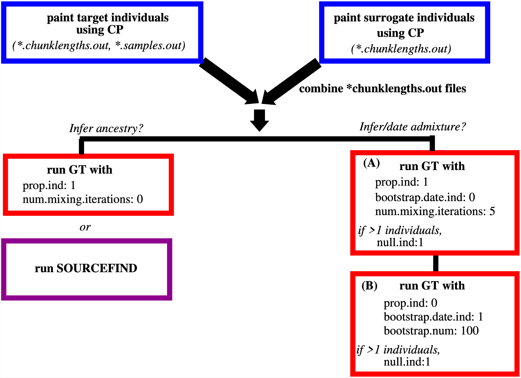
Figure 1. Schematic summarising the steps, parameters and key output files for the ChromoPainter (CP) and GLOBETROTTER/fastGLOBETROTTER (GT) analyses.
The main input for ChromoPainter is the phased haploid genomes of individuals. While most available human datasets consist of individuals’ genotype data without phasing information, several programs exist to infer phasing, such as GLIMPSE [18], IMPUTE [19], BEAGLE [20] and SHAPEIT [21]. After phasing, each diploid individual has two inferred (phased) haploid genomes. ChromoPainterv2, which we use in these examples, comes with a program that converts phased output files from IMPUTE [19] or SHAPEIT [21] into ChromoPainterv2 input files, using the command:
[impute/shapeit genetic map input file] [output file prefix]
To run ChromoPainterv2, the user designates whether phased haploid genomes belong to a “donor” or a “recipient” individual. ChromoPainter independently “paints” each haploid genome of each recipient individual, by inferring the donor haploid that the recipient haploid shares a most recent ancestor with, i.e., a more recent ancestor than it shares with any other donor haploid. The donor haploid for which the recipient haploid shares a most recent ancestor changes along the genome, reflecting historical recombination. In terms of genealogies, ChromoPainter attempts to infer which donor haploid a recipient haploid coalesces with first, out of all donors, which again changes along the recipient genome. To do this inference, ChromoPainter uses a Hidden Markov Model (HMM) based on [22], described in detail in [14]. This model is implemented both in the ChromoPainter software and—with modifications that infer genealogies—in the RELATE/twigSTATs software [23,24].
There are four ChromoPainterv2 input files, described in Table 1.
Table 1. Types of input file used in ChromoPainterv2, with a brief description of each.

The basic usage of ChromoPainterv2 is:
[population label file] -f [recipient/donor assignment file] -o [output file prefix]
As input, fastGLOBETROTTER requires two types of ChromoPainter output. The first contains the inferred total amount of genome-wide DNA that each target and surrogate individual paints against each donor population. The second contains samples from the HMM model for each haploid genome of each target individual, with each sample giving the inferred donor haploid that the target haploid is painted by at each SNP along the genome.
Because it can be parallelised, to save time (and storage space) we typically run ChromoPainter twice for each chromosome. For the first ChromoPainter run, we paint the targets as recipients. For the second ChromoPainter run, we paint the surrogates as recipients, ideally against the same set of donor individuals. (The donors used to paint the surrogates and targets must be closely matched, for reasons explained below.) We give an example command line for each of these two ChromoPainter runs below for the simulated data with one pulse of admixture, using example files provided by the ChromoPainterv2 software.
BrahuiYorubaSimulationChrom22.recomrates -t BrahuiYorubaSimulation.idfile.txt
-f BrahuiYorubaSimulation.poplist.txt 0 0 -s 10 -o
BrahuiYorubaSimulationChrom22
Here “BrahuiYorubaSimulation.poplist.txt” specifies only the simulated target population as a recipient. The ‘-s 10’ above specifies that you want to sample ten paintings from the HMM per each recipient haploid genome. Note that there are additional parameters you can specify for ChromoPainter, with two notable parameters being the average rate at which a recipient switches from matching from one donor to another (specified using ‘-n’) and the allowed rate of allele mis-matches per SNP between a recipient and a donor it is being painted by (specified using ‘-M’). You can also estimate these two parameters using an Expectation-Maximisation algorithm, which is recommended but likely makes little difference in practice over default values, at least when analysing human data.
There are two major output files that fastGLOBETROTTER will use from this analysis.
[BrahuiYorubaSimulationChrom22].chunklengths.out contains the total expected amount of genome in centimorgans (cM) that each recipient individual matches to individuals in each of the donor populations. The sum of the values for each recipient will be two times the total cM length of the chromosome, where the total cM length matches that in the recombination rate file.
[BrahuiYorubaSimulationChrom22].samples.out gives some number (e.g., 10) of painting samples for each recipient haploid genome. Each sample lists which donor haploid the recipient is being painted by at each SNP, inferred by sampling probabilistically from the HMM. An example is given in Figure 2 below.
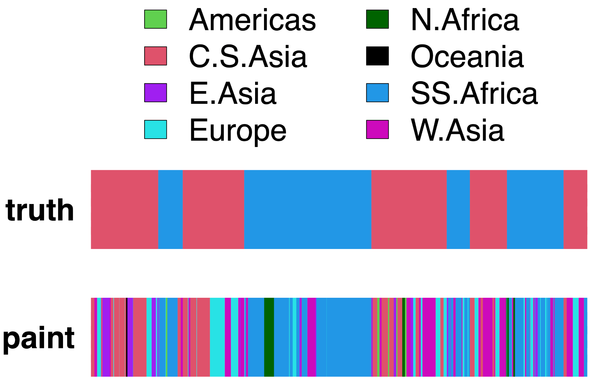
Figure 2. Example of ChromoPainter painting for simulated data. (truth:) The true ancestry assignment for a single recipient haploid from the simulated admixed population, along a region of one chromosome. Here the haploid is a mixture of segments inherited from Yoruba (Sub-Saharan Africa, blue) and Brahui (Central South Asia, red), with segment sizes determined by the simulated admixture date of 30 generations using the technique of [16]. (paint:): One sample of the ChromoPainter HMM for this same recipient haploid in the same region. Colors depict the geographic area (legend at top) of the donor individual that the recipient haploid is painted by along the region.
Intuitively, the main purpose of output file (i) is to help determine which surrogates best represent each admixing source, and at what proportions, as described below. The purpose of the output file (ii) is to date the admixture, by using cM lengths of segments matching to different donor populations.
As seen in Figure 2, the inferred painting from ChromoPainter is quite noisy. While ideally the simulated haploid genomes would be painted only by donors from Sub-Saharan Africa and Central South Asia, as this reflects their true ancestry, in practice they paint segments from donors spanning widely dispersed geographic areas. This is particularly true for segments that are inherited from Central South Asia, which match to several (predominantly non-African) groups.
This noise in the painting can occur for several reasons. First, there will be stochasticity in inference related to the informativeness of the data. For example, if all donors are genetically similar in one region of the genome, perhaps due to sparse SNP data, then ChromoPainter will assign equal weight to each donor in that region. Secondly, for many regions of the genome, the genealogical tree relating sampled individuals back in time is much deeper than the split times between human groups [23]. As a consequence, the donor that a recipient individual shares a most recent ancestor within a genetic region often will not be from the same geographic area that the recipient is from. A third reason is, since ChromoPainter assumes a priori that each donor haploid is equally likely to be painted from, donor populations with more sampled individuals are a priori more likely to be painted from than those with fewer sampled individuals.
For these reasons, using the raw ChromoPainter painting output often will not accurately reflect the true ancestry of an individual. Therefore, fastGLOBETROTTER aims to “correct” the painting by comparing it to the paintings of surrogate populations, with some surrogates hopefully genetically well-representing the ancestral sources of the target group. To do so, we need to paint each surrogate population, using the same set (or a very similar set) of donors. After doing so, fastGLOBETROTTER will assess which surrogate populations have a painting signature that most closely matches that of the target population. The painting signatures of both targets and surrogates should be similarly affected by all of the issues stated above, so this step will in theory alleviate each of these issues.
BrahuiYorubaSimulationChrom22.recomrates -t BrahuiYorubaSimulation.idfile.txt
-f BrahuiYorubaSimulationSURROGATES.poplist.txt 0 0 -o
BrahuiYorubaSimulationChrom22SURROGATES
We have changed three things from the previous command line. First, because we are not dating admixture in the surrogates, we do not require any painting samples, and so “-s 10” has been removed. Secondly, we have changed the output name, so that we do not write over the previous painting results. Third, we have changed the “-f” file, as we are now doing a different painting. In particular the new “-f” file, which is provided with this paper, specifies each surrogate population as recipients (“R”) to be painted against the donors (“D”). Note the 93 donor populations are the same here as in the previous “-f” file we used. Note also that the surrogates are the same as the donors. As a recipient cannot paint against themself, this creates an asymmetry with the painting in (1), as the set of donors a surrogate paints against will not be exactly identical to the set of donors a target paints against (In particular the surrogates will paint against exactly one less donor—themself). In practice, this asymmetry can be problematic if the number of individuals in some populations used as both a donor and surrogate is low (e.g., <5). Otherwise, we typically ignore this asymmetry, as we do here. A more principled approach is to drop one individual from each donor population in the donor set, which enables painting each surrogate and target against exactly the same number of individuals from each donor population. We often refer to this in the literature as a leave-one-out approach [7,25].
For this painting of the surrogates, the only output file we use going forward is the analogue to (i) in the previous section: the [BrahuiYorubaSimulationChrom22SURROGATES].chunklengths.out file. Figure 3 summarises the painting results from this file, though after combining the paintings across all 22 autosomes.
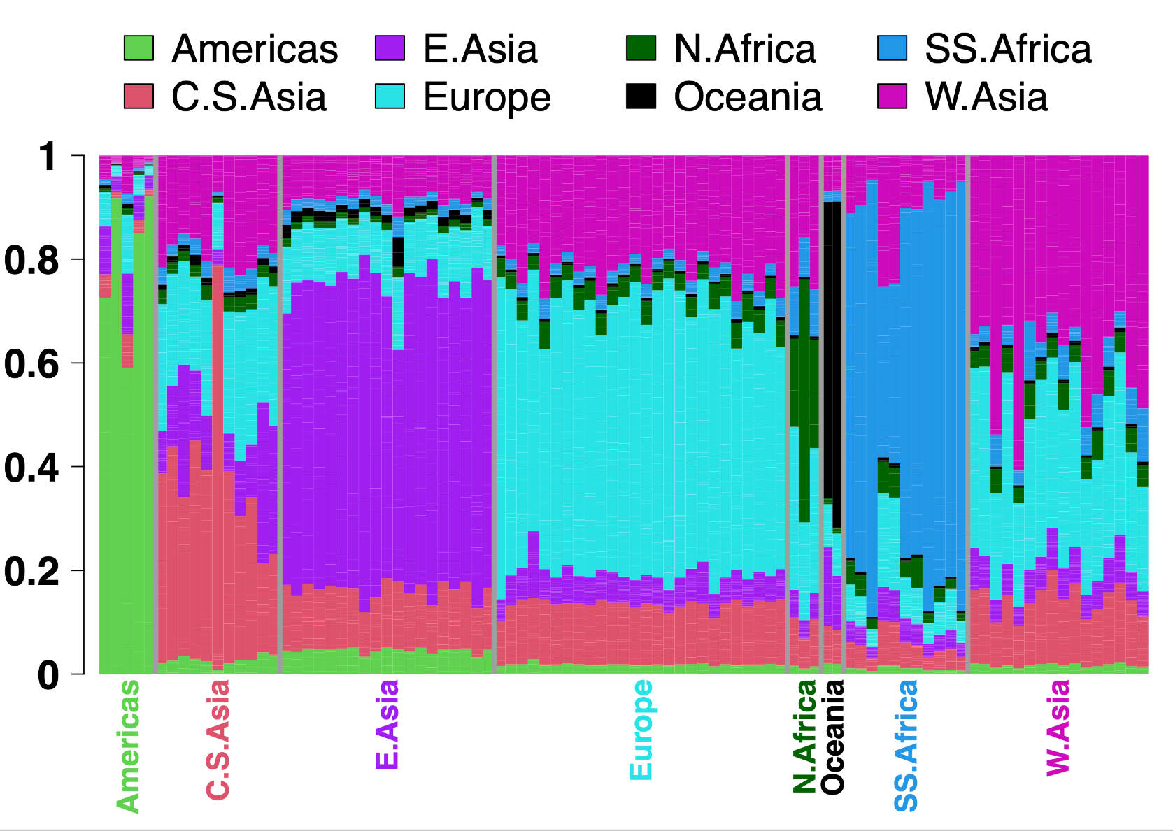
Figure 3. ChromoPainter inferred painting for the 93 surrogate populations. Each bar depicts the proportion of genome-wide DNA for which individuals from the given population are, on average, painted by donors from each of eight worldwide geographic areas (colors). Labels between grey vertical lines give the geographic area each surrogate population is sampled from, with colors corresponding to the legend at top. Note that while the 93 surrogate populations are largely painted by donors from the same geographic area, some parts of their genomes are painted by donors from other areas, analogous to the “noisy” painting seen in Figure 2.
After running the above two paintings for every chromosome, the user should sum the two chunklengths.out matrices across all chromosomes. They should then combine the target and surrogate chunklengths.out files into a single file (with individuals in any order). This gives a final .chunklengths.out file, e.g., “BrahuiYorubaSimulation.copyvectors.txt” described below, that contains the total cM amount of analysed genome that each target individual and each surrogate individual matches to each donor population.
One application of fastGLOBETROTTER is to infer the ancestral composition of a target population, without dating admixture events or even assuming the target population is admixed at all. With this setting, the painting signature of a target population is inferred to be a mixture of those of the surrogate populations, and the program infers the best-fitting mixture proportions.
Specifically, let Yd be the total proportion of genome-wide DNA in a target individual that is painted by some donor d. Analogously, let (X1d,…,XSd ) be the total proportion of genome-wide DNA painted by donor d in surrogate populations 1,…,S, respectively. For example, if d = “Sub-Saharan African” donors, the dark blue proportions in Figure 3 depict (X1d,…,XSd ) for the S=93 surrogate populations. fastGLOBETROTTER assumes that the expected value of Yd, i.e., E[Yd], follows:
Assuming this relationship for all donors d, e.g., each of the colors in Figure 3, the programs infer (β1,…,βS) using non-negative least squares (NNLS), under the restriction that (β1 + … + βS) = 1.0. These (β1,…,βS) reflect a “cleaning” of the painting that is designed to account for the issues described above, and is reported as the inferred ancestral composition of the target individual.
In practice, if a target population has multiple individuals, then Yd is the average painted amount across all individuals for each d, with the Xsd for each surrogate population similarly represented by average values. The donors d are typically defined using group labels, or clusters. For example, the file “BrahuiYorubaSimulation.copyvectors.txt”, provided with the GLOBETROTTER software and used to make Figure 3, contains the *.chunklengths.out output from ChromoPainter for all surrogate and target individuals, i.e., as generated above though here summed across all 22 autosomes. In this file, there are 93 values per each target and surrogate individual, which give the total amount of analysed genome for which that individual is painted by donor individuals from the 93 donor populations.
To infer the ancestry composition for the simulated individuals using GLOBETROTTER, without inferring admixture, the basic command line is:
(In contrast for this scenario, fastGLOBETROTTER requires specifying all parameter files listed below.) There is one required parameter input file, with BrahuiYorubaSimulation.paramfile.txt an example provided to analyse the simulated population. In the input file, the user specifies the donor populations (in the line beginning “copyvector.popnames”), the surrogate populations (“surrogate.popnames”) and the target population (“target.popname”). The user also provides the filename for the [population label file] supplied to ChromoPainter (“input.file.ids”), and the filename for the final *.chunklengths.out output containing painting results for all surrogate and target populations (“input.file.copyvectors”). To infer ancestry composition only, the user must also specify “prop.ind: 1” and “num.mixing.iterations: 0”.
To run on the example file provided with GLOBETROTTER, you then use:
The output file, specified in the line beginning “save.file.main” in the parameter file, gives the inferred (β1,…,βS) values for all surrogates with a β value >0.1%. These results are depicted graphically in Figure 4. Reflecting the simulated truth, here only surrogate populations from Sub-Saharan Africa and Central South Asia have large β values. Furthermore, values across the largest contributing Sub-Saharan African surrogates sum to ~16%, and values across Central South Asian populations sum to ~81%, closely reflecting the true 20% versus 80% mixture.
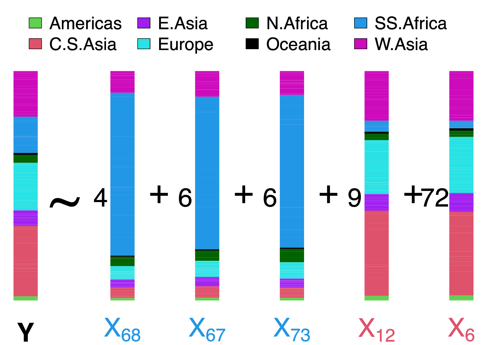
Figure 4. Inferred ancestry composition for the simulated individuals. As in Figure 3, each bar depicts the average proportion of genome-wide DNA for which individuals from the given population are, on average, painted by donors from each of seven worldwide geographic areas (colors). Y refers to the target population, and black numbers give the inferred contribution (i.e., β values) from each surrogate population Xs, whose subscripts correspond to the columns in Figure 3. Note that 97% of the total contribution to Y is inferred to come from only five of the 93 surrogate populations depicted in Figure 3.
An alternative approach SOURCEFIND instead infers the (β1,…,βS) using a Bayesian model that puts a prior probability on the number of surrogates with non-zero β values, which in simulations gives more accurate ancestry estimates (Chacón-Duque et al., 2018). Another difference is that SOURCEFIND assumes that (C*Yd) follows a multinomial distribution with mean C*(β1 * X1d + … + βS * XSd), where C is equal to twice the total length (in centimorgans) of the analysed genome. The SOURCEFIND input and command line is very similar to that for GLOBETROTTER above. Though SOURCEFIND uses an MCMC algorithm that results in an increased runtime, due to its increased accuracy we recommend using it as well when inferring the ancestry composition of a target population.
fastGLOBETROTTER also tests whether a target population is admixed, inferring the date(s) of admixture and the genetic make-up of the admixing sources. Currently the program can infer up to two dates of admixture per target population.
To infer and date admixture, as with other approaches like ALDER [2], DATES [6] and MOSAIC [9], fastGLOBETROTTER leverages signatures of linkage disequilibrium decay in the target individuals that are attributable to admixture. In particular it uses the ChromoPainter *samples.out files, alongside the NNLS procedure described in the previous section, to assign a probability that each segment along a target individual’s genome shares a most recent ancestor with each surrogate population. Then for every pairing of surrogate populations, it calculates the probability that two segments separated by some cM distance have one segment sharing a most recent ancestor with one surrogate in the pair, and the other segment sharing a most recent ancestor with the other surrogate in the pair [7]. These probabilities, referred to as coancestry curves, can be used to infer both the sources and dates of admixture as described below.
Inferring admixture with fastGLOBETROTTER requires three input files, described in Table 2.
Table 2. Types of input file used in fastGLOBETROTTER, with a brief description of each.
The basic command line to run fastGLOBETROTTER is the following:
[recombination rate file list] [option] --no-save > [screen output]
Here we will set the “option” value, which is the only specification in the command line above that is not required when inferring admixture using GLOBETROTTER, to “1”, which will implement the fastest version of fastGLOBETROTTER. When inferring admixture in the target population, there are several parameter options you can specify in the parameter file. We recommend first setting “prop.ind: 1”, “bootstrap.date.ind: 0”, and “num.mixing.iterations: 5”, which will infer admixture dates and sources, separately for two scenarios that assume one versus two dates of admixture. If you have more than one target individual, we also recommend always setting “null.ind: 1”, which leverages patterns of linkage disequilibrium decay among segments from different target individuals to account for potentially false admixture signatures caused by demographic events (e.g., bottlenecks). After running with these parameters, we recommend re-running while setting “prop.ind: 0”, “bootstrap.date.ind: 1”, and “bootstrap.num: 100”. This will use 100 bootstrap re-samples of target individuals to infer confidence intervals around the inferred admixture date(s) generated in the first analysis. (If the results from the first step indicate there genuinely are two distinct dates of admixture, also set “num.admixdates.boostrap: 2” to infer confidence intervals for both dates.) Depending on the computational complexity of the analysis, this second bootstrapping step can be parallelised, for example by running ten separate times with “bootstrap.num: 10”. If you have only a single target individual, you cannot do bootstrap re-sampling; in this case fastGLOBETROTTER has a different jack-knifing procedure to generate confidence intervals around inferred dates. Based on results, two other potentially important parameters to change in this file are “curve.range” and “bin.width”, as we note below.
The example input files provided with GLOBETROTTER analyse only chromosomes 20-22 for the simulated individuals. The following command will analyse these data:
BrahuiYorubaSimulation.samplesfile.txt BrahuiYorubaSimulation.recomfile.txt 1 --no-save > output.out
fastGLOBETROTTER produces four output files, described in Table 3.
Table 3. Types of output file generated by fastGLOBETROTTER, with a brief description of each.
In Figure 5, we describe how to evaluate the results in the admixture description file. Alongside this, we recommend examining figures in the coancestry curves plot file to understand the admixture signal, including assessing whether the conclusions in the admixture description file are consistent with these curves. In particular under a pulse model of admixture, the curves should increase or decrease exponentially, with rate equal to the date(s) of admixture. Therefore, the user should assess whether this is the case. Coancestry curves that clearly increase along with the genetic distance between two segments indicate that the two surrogate populations used to generate the curves represent different sources of admixture. In contrast, coancestry curves that clearly decrease with increasing genetic distance indicate the two surrogate populations represent the same admixing source. Therefore, the curves can be assessed to check which surrogate populations best reflect each admixing source, and the evidence for more than two admixing sources.
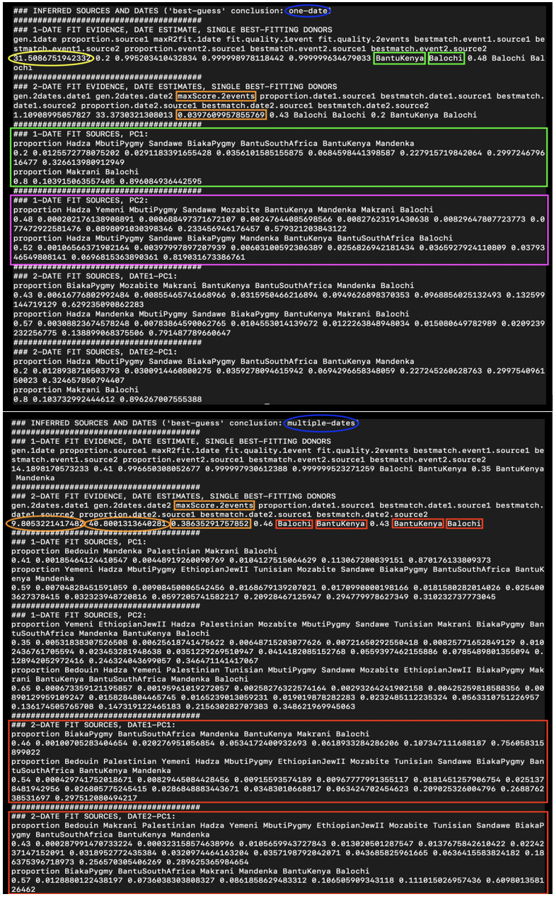
Figure 5. Examples of *.main.txt output files from fastGLOBETROTTER, for the simulations with one pulse (top) and two pulses (bottom) of admixture. FastGLOBETROTTER’s best-guess conclusion for the type of admixture in each case is given at top (blue circles), with inferred dates when assuming either one date (yellow circle) or two dates of admixture (orange circle) given underneath this. Concluding “multiple-dates” is based on “maxScore.2events” (orange box) being >=0.35, a threshold chosen based on simulated results [7]. As “one-date” is inferred in the top case, we use the yellow circle, and we use the inference in the green boxes to describe (top green box) the surrogate population that is inferred to be most genetically similar to each admixing source and (bottom green box) the proportions contributed by each of the two admixing sources and each source’s inferred genetic make-up. This genetic make-up is described as a mixture of the surrogates by using the model illustrated in Figure 4. (If “one-date-multiway” is inferred, indicating >2 sources intermixing around the same time, we also use the inference in the purple box, but that is not the case here.) As “multiple-dates” is inferred in the bottom case, we instead use the orange circle, and we use the inference in the red boxes to describe the inferred sources and proportions, separately for the first inferred admixture date (underneath “2-DATE FIT SOURCES, DATE1-PC1”, representing the inferred date “gen.2dates.date1” at top) and for the second inferred admixture date (underneath “2-DATE FIT SOURCES, DATE2-PC1”, representing the inferred date “gen.2dates.date2” at top).
To provide some intuition, consider that for an admixture event between populations A and B occurring r generations ago under fastGLOBETROTTER’s assumptions, the probability Pr(x,y) that two segments separated by d Morgans within an admixed individual’s genome are inherited from populations {x,y} ∈ {A,B} is:
with α the proportion of DNA contributed by population A, and γ=α if x=A or γ=(1-α) if x=B [7]. Note that Pr(x,y) decreases with d if x=y=A or x=y=B, i.e., when the two segments are inherited from the same admixing source. In contrast, Pr(x,y) increases with d if x=A and y=B, i.e., when the two segments are inherited from different admixing sources.
Finally, the user should check whether the model assuming two dates of admixture fits the curves substantially better than the model assuming only one date; if not, the one date fit is a more parsimonious solution.
Example output from the admixture description and coancestry curve plots files for both simulated target populations, when analysing each using all 22 autosomes, are provided in Figures 5 and Figures 6. In the case of the simulation with one pulse of admixture, the inference assuming one date of admixture seems to sufficiently fit the data. The rate of these exponential curves is ~31, which is close to the true admixture date of 30 generations. In addition, the surrogate population Balochi, sampled from Central South Asia, has an increasing coancestry curve when paired with any of the surrogate populations sampled in Sub-Saharan Africa, including the Mandenka. In contrast, all pairings of the surrogate populations from Sub-Saharan Africa, such as BantuKenya and Mandenka, have decreasing curves. This accurately reflects how the simulated admixture is between Central South Asian and Sub-Saharan African sources.
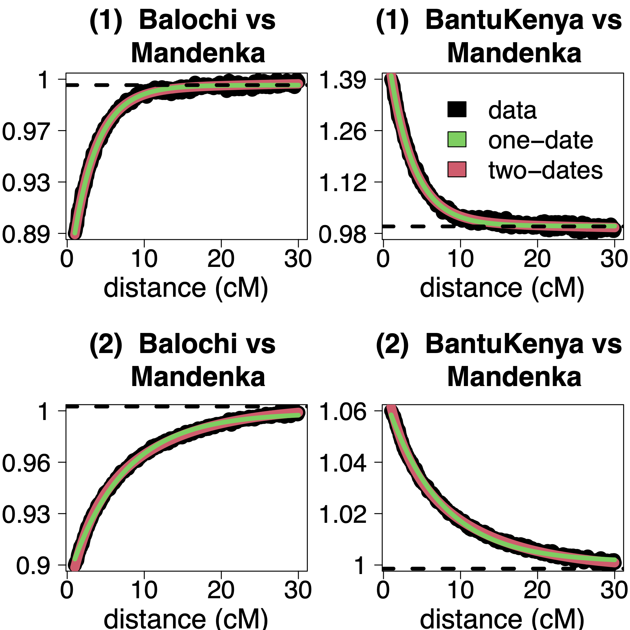
Figure 6. Example coancestry curves for the simulated data with (top row) one date and (bottom row) two dates of admixture. In each plot, black lines give the scaled probability (y-axis) that two segments in a target individual’s genome separated by a given distance (x-axis) are most recently related to the two surrogate populations listed in the title. Green lines give the fit of the model assuming one date of admixture, while red lines give the fit assuming two dates of admixture.
For the simulated data with two pulses of admixture (i.e., an additional pulse of Yoruban admixture), now the fit of two dates (red line in Figure 6) appears to be a subtly better fit to the data than the fit of one date (green line). This is reflected in the output from the admixture description file, which concludes two dates of admixture at ~10 and ~41 generations ago. However, inferring the older date can be challenging, as the first date can mask it – even with 150 simulated individuals, the fit of two dates is very similar to the fit of one date in Figure 6.
Finally, for the single-date simulation scenario, the scaled probabilities are flat when the distance between the two segments exceeds 10cM. The model fits all pairs of segments within the range specified by “curve.range” in the parameter file, which by default is all segments separated by >1cM and <30cM. For this reason, it would be sensible to re-run fastGLOBETROTTER after setting “curve.range” to instead fit curves separated by >1cM and <10cM in this case, as the model is only fitting random noise in segments separated by >10cM. If necessary, “bin.width” can be adjusted alongside “curve.range” to control the number of distance bins used to build the coancestry curves.
While here we illustrate how ChromoPainter combined with fastGLOBETROTTER can accurately infer and date admixture in simulated examples, this protocol has some important limitations. For example, the sizes of segments inherited from each admixing source decrease with time due to recombination. Hence older admixture dates, e.g., occurring over 150-200 generations prior to the age of the target population, may be difficult to detect. While this issue affects all admixture inference approaches that leverage the decay of linkage disequilibrium related to admixture, including ALDER [2] and MOSAIC [9], alternative approaches such as f3-statistics [5] should be more robust to admixture age.
In addition, currently fastGLOBETROTTER can only describe up to two dates of admixture per target population. As with many other methods [2-6,9] they assume admixture occurs in “pulses”, which is an over-simplification [26].
In particular, admixture in many cases likely occurs over several years and overlapping generations. Indeed in practice we suggest that if these programs infer two dates of admixture involving the same sources in a target population, this is reported as potentially reflecting continuous admixture spanning the two inferred dates.
Even more complicated are cases where more than two sources intermixed, at the same or different times, in the history of a target population, which is highly plausible given the complex series of interactions throughout human history. While fastGLOBETROTTER can test for >2 intermixing sources, it does not fully attempt to describe the genetic make-up of each source in such cases. Instead they describe signatures in the admixture patterns that require further interpretation from the user, e.g., through studying the coancestry curves as described above. Other approaches attempt to model more complicated admixture histories, e.g., using Approximate-Bayesian-Computation (ABC) techniques [27].
If an admixing group is not well reflected by any surrogate population, the signal of admixture can weaken. When admixture is inferred, a sign of having no good representative surrogate for a source is if several geographically disparate surrogates are used to describe that source. A separate issue occurs if a surrogate is too closely genetically related to the target population, which may mask any (potentially shared) admixture events. Fortunately, this is relatively easy to diagnose and resolve, as the target should match almost entirely to this surrogate population in the NNLS analysis. In such cases, the surrogate population can be removed before re-running. To avoid computational hassle, ideally fastGLOBETTER can be re-run without having to re-run ChromoPainter, e.g., by keeping the offending population as a donor while removing them as a surrogate. However, a better strategy is to remove this population as a donor and re-paint, as keeping them as a donor may in particular act to mask the signal of any admixture when generating the *samples.out files for the target population. Such a re-painting may be helpful if the reported best-guess admixture conclusion is “unclear signal”.
fastGLOBETROTTER relies on ChromoPainter output to infer admixture. While recipient individuals tend to be painted by many world-wide donor populations (e.g., Figure 2-3), they typically are painted more by the donors they are most closely related to genetically than any other group is painted by those same donors. For example, relative to any non-African surrogate population, Sub-Saharan African surrogates are painted considerably more by Sub-Saharan African donors (Figure 3). This reflects population-specific (or region-specific) levels of genetic drift. However, when surrogate and donor populations overlap, which is often the case in practice, there are some subtle issues that can arise due to differences among these populations’ sample sizes, even after attempting to correct for sample size using e.g., NNLS. In particular surrogate populations with small sample sizes are less able to capture population-specific drift, since they have fewer donors to paint against. In an extreme (yet realistic) case where a surrogate population has only one individual, it cannot paint against any donors from its own population. A consequence is that surrogates with such small sample sizes, perhaps <5 individuals in practice, may tend to be over-represented among the inferred ancestry sources of target populations. The reason for this is that a lack of a “unique” drift signature in such surrogates could make them seem more genetically similar to the true admixing sources than would be the case if this drift were better captured. Ensuring surrogate populations have similar sample sizes should mitigate any such issues.
Overall, since available programs have varying strengths and weaknesses, we recommend running multiple software (e.g., ALDER, MOSAIC) and assessing consistency across findings when reporting results. Despite their difficulties, these programs have proven to be powerful tools to detect admixture in a variety of settings, and will hopefully continue to assist with further insights into the history of humans and other organisms.
Not applicable.
Not applicable.
Code used here and some data is available at https://github.com/hellenthal-group-UCL. Full data is available at https://data.mendeley.com/datasets/ckz9mtgrjj/1.
GH is supported by a Wellcome Trust Senior Research Fellowship (224575/Z/21/Z). MC is supported by the UCL Research Excellence Scholarship.
The authors have declared that no competing interests exist.
| 1. | Falush D, Stephens M, Pritchard JK. Inference of population structure using multilocus genotype data: linked loci and correlated allele frequencies. Genetics. 2003;164(4):1567-1587. [Google Scholar] [CrossRef] |
| 2. | Loh P-R, Lipson M, Patterson N, Moorjani P, Pickrell JK, Reich D, et al. Inferring admixture histories of human populations using linkage disequilibrium. Genetics. 2013;193(4):1233-1254. [Google Scholar] [CrossRef] |
| 3. | Pickrell JK, Patterson N, Loh P-R, Lipson M, Berger B, Stoneking M, et al. Ancient west Eurasian ancestry in southern and eastern Africa. Proc Natl Acad Sci USA. 2014;111(7):2632-2637. [Google Scholar] [CrossRef] |
| 4. | Moorjani P, Patterson N, Hirschhorn JN, Keinan A, Hao L, Atzmon G, et al. The history of African gene flow into Southern Europeans, Levantines, and Jews. PLoS Genet. 2011;7(4):e1001373. [Google Scholar] [CrossRef] |
| 5. | Patterson N, Moorjani P, Luo Y, Mallick S, Rohland N, Zhan Y, et al. Ancient admixture in human history. Genetics. 2012;192(3):1065-1093. [Google Scholar] [CrossRef] |
| 6. | Chintalapati M, Patterson N, Moorjani P. The spatiotemporal patterns of major human admixture events during the European Holocene. Elife. 2022;11:e77625. [Google Scholar] [CrossRef] |
| 7. | Hellenthal G, Busby GB, Band G, Wilson JF, Capelli C, Falush D, et al. A genetic atlas of human admixture history. Science. 2014;343(6172):747-751. [Google Scholar] [CrossRef] |
| 8. | Wangkumhang P, Greenfield M, Hellenthal G. An efficient method to identify, date, and describe admixture events using haplotype information. Genome Res. 2022;32(8):1553-1564. [Google Scholar] [CrossRef] |
| 9. | Salter-Townshend M, Myers S. Fine-scale inference of ancestry segments without prior knowledge of admixing groups. Genetics. 2019;212(3):869-889. [Google Scholar] [CrossRef] |
| 10. | Van Dorp L, Balding D, Myers S, Pagani L, Tyler-Smith C, Bekele E, et al. Evidence for a common origin of blacksmiths and cultivators in the Ethiopian Ari within the last 4500 years: lessons for clustering-based inference. PLoS Genet. 2015;11(8):e1005397. [Google Scholar] [CrossRef] |
| 11. | Busby GB, Hellenthal G, Montinaro F, Tofanelli S, Bulayeva K, Rudan I, et al. The role of recent admixture in forming the contemporary West Eurasian genomic landscape. Curr Biol. 2015;25(19):2518-2526. [Google Scholar] [CrossRef] |
| 12. | Moorjani P, Hellenthal G. Methods for assessing population relationships and history using genomic data. Annu Rev Genomics Hum Genet. 2023;24(1):305-332. [Google Scholar] [CrossRef] |
| 13. | Wangkumhang P, Hellenthal G. Statistical methods for detecting admixture. Curr Opin Genet Dev. 2018;53:121-127. [Google Scholar] [CrossRef] |
| 14. | Lawson DJ, Hellenthal G, Myers S, Falush D. Inference of population structure using dense haplotype data. PLoS Genet. 2012;8(1):e1002453. [Google Scholar] [CrossRef] |
| 15. | Chacón-Duque J-C, Adhikari K, Fuentes-Guajardo M, Mendoza-Revilla J, Acuña-Alonzo V, Barquera R, et al. Latin Americans show wide-spread Converso ancestry and imprint of local Native ancestry on physical appearance. Nat Commun. 2018;9(1):5388. [Google Scholar] [CrossRef] |
| 16. | Price AL, Tandon A, Patterson N, Barnes KC, Rafaels N, Ruczinski I, et al. Sensitive detection of chromosomal segments of distinct ancestry in admixed populations. PLoS Genet. 2009;5(6):e1000519. [Google Scholar] [CrossRef] |
| 17. | Li JZ, Absher DM, Tang H, Southwick AM, Casto AM, Ramachandran S, et al. Worldwide human relationships inferred from genome-wide patterns of variation. Science. 2008;319(5866):1100-1104. [Google Scholar] [CrossRef] |
| 18. | Rubinacci S, Ribeiro DM, Hofmeister RJ, Delaneau O. Efficient phasing and imputation of low-coverage sequencing data using large reference panels. Nat Genet. 2021;53(1):120-126. [Google Scholar] [CrossRef] |
| 19. | Marchini J, Howie B, Myers S, McVean G, Donnelly P. A new multipoint method for genome-wide association studies by imputation of genotypes. Nat Genet. 2007;39(7):906-913. [Google Scholar] [CrossRef] |
| 20. | Browning SR, Browning BL. Rapid and accurate haplotype phasing and missing-data inference for whole-genome association studies by use of localized haplotype clustering. Am J Hum Genet. 2007;81(5):1084-1097. [Google Scholar] [CrossRef] |
| 21. | Delaneau O, Marchini J, Zagury J-F. A linear complexity phasing method for thousands of genomes. Nat Methods. 2012;9(2):179-181. [Google Scholar] [CrossRef] |
| 22. | Li N, Stephens M. Modeling linkage disequilibrium and identifying recombination hotspots using single-nucleotide polymorphism data. Genetics. 2003;165(4):2213-2233. [Google Scholar] [CrossRef] |
| 23. | Speidel L, Forest M, Shi S, Myers SR. A method for genome-wide genealogy estimation for thousands of samples. Nat Genet. 2019;51(9):1321-1329. [Google Scholar] [CrossRef] |
| 24. | Speidel L, Silva M, Booth T, Raffield B, Anastasiadou K, Barrington C, et al. High-resolution genomic history of early medieval Europe. Nature. 2025;637(8044):118-126. [Google Scholar] [CrossRef] |
| 25. | Yang Y, Durbin R, Iversen AK, Lawson DJ. Sparse haplotype-based fine-scale local ancestry inference at scale reveals recent selection on immune responses. Nat Commun. 2025;16(1):2742. [Google Scholar] [CrossRef] |
| 26. | Liang M, Nielsen R. The lengths of admixture tracts. Genetics. 2014;197(3):953-967. [Google Scholar] [CrossRef] |
| 27. | Fortes-Lima CA, Laurent R, Thouzeau V, Toupance B, Verdu P. Complex genetic admixture histories reconstructed with Approximate Bayesian Computation. Mol Ecol Resour. 2021;21(4):1098-1117. [Google Scholar] [CrossRef] |

![]()
Copyright © 2026 Pivot Science Publications Corp. - unless otherwise stated | Terms and Conditions | Privacy Policy


