The quantitative genetics of human disease: 1. Foundations

David J. Cutler; Kiana Jodeiry; Andrew J. Bass; Michael P. Epstein

doi:10.47248/hpgg2303040007

Sections

Abstract
1. Introduction
2. Materials and Methods
3. Results and Discussion
4. Conclusions
Declarations
Reference

Human Population Genetics and Genomics 2023;3(4):0007 | https://doi.org/10.47248/hpgg2303040007

Original Research Open Access

The quantitative genetics of human disease: 1. Foundations

David J. Cutler ^1,2 , Kiana Jodeiry ^2,3 , Andrew J. Bass ^1,2,† , Michael P. Epstein ^1,2

1. Department of Human Genetics, Emory University, Atlanta, GA 30322, USA
2. Center of Computational and Quantitative Genetics, Emory University, Atlanta, GA 30322, USA
3. Department of Psychology, Emory University, Atlanta, GA 30322, USA

† Current address: Department of Medicine, University of Cambridge, Addenbrooke’s Hospital, Hills Road, Cambridge CB2 2QQ, UK

Correspondence: David J. Cutler

Academic Editor(s): Joshua Akey

Received: Aug 8, 2023 | Accepted: Nov 22, 2023 | Published: Dec 7, 2023

© 2023 by the author(s). This is an Open Access article distributed under the terms of the Creative Commons License Attribution 4.0 International (CC BY 4.0), which permits unrestricted use, distribution, and reproduction in any medium or format, provided the original work is correctly credited.

Cite this article: Cutler D, Jodeiry K, Bass A, Epstein M. The quantitative genetics of human disease: 1. Foundations. Hum Popul Genet Genom 2023; 3(4):0007. https://doi.org/10.47248/hpgg2303040007

Abstract

In this the first of an anticipated four paper series, fundamental results of quantitative genetics are presented from a first principles approach. While none of these results are in any sense new, they are presented in extended detail to precisely distinguish between definition and assumption, with a further emphasis on distinguishing quantities from their usual approximations. Terminology frequently encountered in the field of human genetic disease studies will be defined in terms of their quantitive genetics form. Methods for estimation of both quantitative genetics and the related human genetics quantities will be demonstrated. The principal target audience for this work is trainees reasonably familiar with population genetics theory, but with less experience in its application to human disease studies. We introduce much of this formalism because in later papers in this series, we demonstrate that common areas of confusion in human disease studies can be resolved be appealing directly to these formal definitions. The second paper in this series will discuss polygenic risk scores. The third paper will concern the question of “missing” heritability and the role interactions may play. The fourth paper will discuss sexually dimorphic disease and the potential role of the X chromosome.

Background: With over a hundred years of history, most fundamental results in quantitative genetics are well known to most population genetics students, yet there is often considerable confusion concerning precise definitions and assumptions, particularly when interactions may exist. The connections between quantitative genetics and human disease genetics can be obscure to many.

Methods: Fundamental quantitative genetics quantities are derived as conditional expectations of phenotype. Genetic, environmental, additive, dominance and interaction effects and their associated variances are defined, with key results explicitly derived. The effects of linkage disequilibrium and methods to account for it are examined. Methods to estimate and interpret heritability are discussed.

Results: Application of quantitative genetics quantities are extended to binary traits with special emphasis on translation between commonly estimated human disease genetics quantities and their corresponding quantitative genetics representations.

Conclusions: The distinction between modeling definitions and assumptions is made clear. Methods to unite human disease genetics and quantitative genetics are elucidated. Methods to account for linkage disequilibrium and other forms of interaction are described.

Keywords

quantitative genetics, human disease, linkage disequilibrium, liability model, genetic interaction

1. Introduction

Arguably the most important paper in the history of population genetics theory was Fisher 1918, “The Correlation between Relatives on the Supposition of Mendelian Inheritance.” [1]. In this work, nearly impenetrable to read by modern standards, Fisher established the fundamental model of quantitative genetics, unified the seemingly incompatible genetical models of Mendel and Galton, derived heritability from first principles, showed how to predict the correlation between relatives as a function of heritability, and began the process of defining and formalizing analysis of variance [2]. All told, not a bad accomplishment for a work begun as an undergraduate that may have been in revision or “review” for the better part of 8 years [3].

Buried at the heart of Fisher’s model is the idea of the effect of an allele on the phenotype of an individual. In Fisher’s presentation, and subsequent presentations by Falconer [4] and many others [5, 6], the effect of an allele on phenotype is imagined as a physically determined entity - an allele with an effect two millimeters on height transmits two millimeters of height to an offspring when inherited from a parent. The effect of the allele is in some sense immutable, independent of its context or how it is observed. We can think of this interpretation of an allele as analogous to the classical mechanical interpretation of the atom. An electron has energy, spin or position that is determined at all times. In Kempthorne’s 1955 [7] derivation of fundamental quantitative genetics results, he introduces a subtly different interpretation of the effect of an allele. Analogous to the Copenhagen interpretation of the atom where an electron’s state is only determined when acted upon by external forces such as observation, in the Kempthorne presentation, the effect of an allele is fundamentally interactive and probabilisitic. It is only determined once it is in the presence of other genetic and environmental effects in the individual who harbors that allele, and as a result the contribution it makes to phenotype only takes an observable form in the context of these other factors. In different contexts an allele has different effects. Because an allele makes no single determined contribution to phenotype, its effect is defined as the average contribution it makes over all the contexts in which it occurs. To be precise, a genetic effect is defined as the average phenotype of an individual with a given genotype, i.e., an effect is defined as a conditional expectation of phenotype. In any particular person, their height is determined by the allele in question together with all the other genes and environments affecting height, and it is possible that no two individuals are affected exactly the same way by the same allele, because everyone may have some differing combination of genetic and environmental factors. The effect of the allele in question is defined as the average height of individuals with that allele. Thus, an effect is defined to be a conditional expectation, a scalar – as are effects in the Fisher/Falconer interpretation – but here the scalar is determined by the average phenotype of people with that allele, rather than as a fixed, immutable quantity. In individuals with a different collection of other genetic and environmental factors, the effect of this allele could be different. In the “infinitesimal” limit imagined by Fisher/Falconer, where individual effects are so small as to be nearly unmeasurable, there is likely no practical difference between the Fisher/Falconer and Kempthorne interpretations of a genetic effect. In the context of 21^st century human genetics, where the goal of an experiment is often to accurately measure the genetic effect of an allele, the distinction between the these two interpretations will be seen to lie at the crux of many of the most apparently confounding observations. Paper two in this series will make abundantly clear why focus on this subtle distinction can have profound effects on our understanding of human genetics.

For all that follows in these series of papers, we will follow the Kempthorne interpretation of genetic effects. We do so for several reasons. First, in the opinion of these authors, Kempthorne’s approach is, in some sense, more biologically realistic. Almost everything in biology seems interconnected with other elements. It seems more plausible that an allele only affects phenotype in the context of all other genetic/environmental factors than an allele has a predetermined, knowable effect on phenotype that will be exactly the same in two or more different contexts. Second, we favor the Kempthorne interpretation for its modeling elegance and ease of presentation. This framework allows use to clearly delineate model assumptions, and it will become obvious that very few assumptions are necessary for virtually all quantitative genetics to be well-defined and interpretable. It is in this framework that higher order interactions become most easy to understand. Finally, and of most practical utility, we will see over the course of all four papers that the Kempthorne interpretation will help us to better understand numerous perplexing observations in human genetics, while giving us analytical tools to confront those challenges.

2. Materials and Methods

The presentation below largely follows Kempthorne, 1955, in a somewhat more modern notation, with much greater detail to assist the student in understanding results. While the formalism is strictly Kempthorne’s, in only a very few places does the distinction between the Kempthorne and Fisher/Falconer interpretation lead to any material difference in how a result is viewed or understood. In those cases we will endeavor to point out what implications the differing interpretations have. Throughout this section we will refer to the Fisher/Falconer interpretation of genetic effect as the Falconer interpretation as his detailed derivations, presentations, and formalism are far more commonly read by population geneticists than Fisher’s. In our first simplification from Kempthorne, we restrict our presentation to only two alleles at each locus because in a modern context we think of these loci as single nucleotide changes, single nucleotide polymorphisms (SNP) in the usual term of human genetics, rather than a more abstract concept like gene or locus that Kempthorne envisioned nearly 70 years ago.

2.1 Single locus

To begin, consider a single diploid locus in Hardy-Weinberg equilibrium with two alleles A₀ and A₁, where the frequency of A₀ is p, and the frequency of A₁ is q = 1 − p. For the sake of notational convenience let us suppose that we have oriented the allelic labels such that p ≥ q. Thus, in the parlance of human genetics, A₀ is the “major” allele, and A₁ is the “minor” allele. Imagine individuals have some observable, measurable quantitative phenotype Y such as height, weight, or blood pressure. Further suppose that individuals with genotype A₀A₀ have average phenotype y₀₀, individuals with genotype A₀A₁ have average phenotype y₀₁, and individuals with genotype A₁A₁ have average phenotype y₁₁. Thus,

\begin{array}{l} E [Y | G = A_{0} A_{0}] & = & y_{00} . \\ E [Y | G = A_{0} A_{1}] & = & y_{01} . \\ E [Y | G = A_{1} A_{1}] & = & y_{11} . \\ μ_{y} = E [Y] & = & Pr [G = A_{0} A_{0}] E [Y | G = A_{0} A_{0}] \\ + Pr [G = A_{0} A_{1}] E [Y | G = A_{0} A_{1}] \\ + Pr [G = A_{1} A_{1}] E [Y | G = A_{1} A_{1}] \\ = & p^{2} y_{00} + 2 p q y_{01} + q^{2} y_{11} . \end{array}

The overall population mean is thus found by appeal to the law of total expectation: the expectation of random variable X is the ΣPr[X = x]E[X|X = x], where the sum is taken over all possible states x of the random variable X. For computational tractability, instead of working with phenotype Y, we will instead consider the linear transformation of Y, P, where P = Y – μ_y. Thus, P is a zero centered translation of Y. We have made this transformation so that P has mean 0, E[P] = E[Y – μ_y] = E[Y] – μ_y = 0, but otherwise the shape of P’s distribution is the same as Y’s. We call P the phenotype of an individual. That P has mean 0 will be used repeatedly in all that follows.

Define the “genetic effects” γ₀₀,γ₀₁,γ₁₁ of genotypes A₀A₀, A₀A₁, A₁A₁ to be the average phenotype of individuals with those genotypes, i.e., the conditional expectation of phenotype given the genotype. If we let G be the two allele genotype at this locus

\begin{array}{l} γ_{00} & = & E [P | G = A_{0} A_{0}] . \\ γ_{01} & = & E [P | G = A_{0} A_{1}] . \\ γ_{11} & = & E [P | G = A_{1} A_{1}] . \\ E [P] & = & Pr [G = A_{0} A_{0}] E [P | G = A_{0} A_{0}] + Pr [G = A_{0} A_{1}] E [P | G = A_{0} A_{1}] \\ + Pr [G = A_{1} A_{1}] E [P | G = A_{1} A_{1}] \\ = & p^{2} γ_{00} + 2 p q γ_{01} + q^{2} γ_{11} = 0. \end{array}

Thus, the genetic effect of genotype G = A_iA_j, i,j ∈{0,1}, is given by γ_ij, which is the conditional expectation of phenotype, given the individual has genotype A_iA_j. Notice that if two populations have differing genotype frequencies at this locus, the genetic effects are necessarily different, since both populations will have been normalized to have mean zero phenotype. Here we see the first element of the difference between the Falconer and Kempthorne interpretations. A Falconer view point might imagine the genetic effects as fixed and independent of allele frequencies. In Kempthorne’s approach genetic effects are only defined conditional on the genotype frequencies.

In a similar fashion, call the “allelic effect” the conditional expectation of phenotype, given an individual possesses the allele. Let α₀ and α₁ be the allelic effects of A₀ and A₁. To find α₀ imagine picking an individual at random from the population. Next imagine picking an allele at random from the chosen person. The probability that the chosen allele was A₀ is, by definition, p. Similarly, the probability the picked allele was A₁ is q. We find the allelic effect α as the conditional expectation of phenotype given the picked allele. Let A be a randomly picked allele

\begin{array}{l} α_{0} & = & E [P | A = A_{0}] \\ = & Pr [G = A_{0} A_{0} | A = A_{0}] E [P | G = A_{0} A_{0}] \\ + Pr [G = A_{0} A_{1} | A = A_{0}] E [P | G = A_{0} A_{1}] \\ + Pr [G = A_{1} A_{1} | A = A_{0}] E [P | G = A_{1} A_{1}] \\ = & \frac{p^{2}}{p} γ_{00} + \frac{1}{2} \frac{2 p q}{p} γ_{01} + 0 \\ = & p γ_{00} + q γ_{01} . \\ α_{1} & = & E [P | A = A_{1}] \\ = & p γ_{01} + q γ_{11} . \end{array}

Importantly, note that from these definitions

\begin{array}{l} p α_{0} + q α_{1} & = & p (p γ_{00} + q γ_{01}) + q (p γ_{01} + q γ_{11}) \\ = & p^{2} γ_{00} + 2 p q γ_{01} + q^{2} γ_{11} = 0. \\ α_{0} & = & \frac{- q α_{1}}{p} . \\ α_{1} & = & \frac{- p α_{0}}{q}, \end{array}

further reenforcing the notion that in the Kempthorne framework the allelic effects are defined in terms of the allele frequencies. At first this might sound counter-intuitive, but there is a natural way to understand this. In the Kempthorne framework, the effect of an allele is determined by the average phenotype of individuals with that allele where the average is taken over all the other genetic and environmental contexts the allele occurs. If heterozygotes and homozygotes have different average phenotypes, then the frequency with which an allele is in those two different contexts is a function of the allele frequency, and the effect of an allele is dependent on its frequency. We define a related variable β = α₁ – α₀ as the difference in the allelic effects between the two alleles. This variable β is naturally interpreted as the consequence of substituting an A₁ allele for an A₀ allele, and will be commonly estimated in a linear regression or related framework. We will discuss in much greater detail in paper two how β could be, and very likely often is, independent of allele frequency.

While formally we define α as an allelic effect (mean phenotype of an individual with that allele), we will often refer to α’s as the “additive effect” of an allele, and may frequently use the terms “allelic effect” and “additive effect” interchangeably. At first blush this interchange of terms may seem very odd. Traditionally in one locus population genetics the term “additive” is used to describe a dominance relationship. A locus is called additive when the phenotype of the heterozygote is the average of the two homozygous phenotypes. In this context, a locus is additive if $γ_{01} = \frac{γ_{00} + γ_{11}}{2}$ . It turns out that there is a very natural reason to equate the terms “allelic effects” and “additive effects.” Note that if the locus is additive then

\begin{array}{l} 0 & = & p^{2} γ_{00} + 2 p q γ_{01} + q^{2} γ_{11} \\ = & p^{2} γ_{00} + 2 p q (γ_{00} + γ_{11}) / 2 + q^{2} γ_{11} \\ = & γ_{00} (p^{2} + p q) + γ_{11} (p q + q^{2}) \\ = & γ_{00} p (p + q) + γ_{11} q (p + q) \\ = & p γ_{00} + q γ_{11} \\ 2 α_{0} & = & 2 p γ_{00} + 2 q γ_{01} \\ = & 2 p γ_{00} + 2 q (γ_{00} + γ_{11}) / 2 \\ = & p γ_{00} + q γ_{00} + p γ_{00} + q γ_{11} \\ = & γ_{00} (p + q) + 0 \\ = & γ_{00} \\ α_{0} + α_{1} & = & p γ_{00} + q γ_{01} + p γ_{01} + q γ_{11} \\ = & p γ_{00} + γ_{01} (p + q) + q γ_{11} \\ = & (p γ_{00} + q γ_{11}) + γ_{01} \\ = & γ_{01} \\ 2 α_{1} & = & 2 p γ_{01} + 2 q γ_{11} \\ = & 2 p (γ_{00} + γ_{11}) / 2 + 2 q γ_{11} \\ = & p γ_{00} + p γ_{11} + q γ_{11} + q γ_{11} \\ = & (p γ_{00} + q γ_{11}) + γ_{11} (p + q) \\ = & 0 + γ_{11} = γ_{11} . \end{array}

Thus, we find for an additive locus the total genetic effects are simply the sum of the individual allele effects added together. For such an additive locus

\begin{array}{l} γ_{00} & = & 2 α_{0} . \\ γ_{01} & = & α_{0} + α_{1} . \\ γ_{11} & = & 2 α_{1} . \end{array}

In a Falconer inspired presentation of this work, one might have been asked to assume that the total genetic effect at a locus was the sum of the individual “additive” effects of the alleles. This could be an assumption of the model. In a Kempthorne framework, where the definition of allelic effects are the mean phenotype of individuals with that allele, for any locus in Hardy-Weinberg that is additive, additivity implies that the genotype effect is the sum of the allelic effects. For an additive locus, the genotype effect is simply the sum of its individual allelic effects. For a non-additive locus, the genotypic effects will differ from the sum of the allelic effects. Let δ be the difference between the genetic effects of a genotype from the sum of its individual allelic effects. In particular, let

\begin{array}{l} δ_{00} & = & γ_{00} - 2 α_{0} . \\ γ_{00} & = & 2 α_{0} + δ_{00} . \\ δ_{01} & = & γ_{01} - (α_{0} + α_{1}) . \\ γ_{01} & = & α_{0} + α_{1} + δ_{01} . \\ δ_{11} & = & γ_{11} - 2 α_{1} . \\ γ_{11} & = & 2 α_{1} + δ_{11} . \end{array}

We will frequently call δ_ij the “dominance deviation” of genotype A_iA_j. Now, imagine a random variable, g, representing the genetic effect of this locus, where its value is determined by the genotype of an individual. Thus if an individual has genotype G = A_iA_j, then g = γ_ij. Genotype is viewed as a randomizing process, and when G = A_iA_j a random variable g has value γ_ij. This random variable g can be further decomposed into a random variable a, whose value is the sum of the allelic effects a = α_i + α_j, and another random variable d = δ_ij, the deviation (difference) from additivity due to dominance. In all cases we think of these random variables, g,a,d, as being determined by the random process of genotype in the individual. Thus, in a notational convention we will attempt to maintain throughout, G refers to a randomly determined genotype with effect, average phenotype conditional on the genotype, γ. A refers to a random allele, with effect, average phenotype conditional on the allele, α. The lower case g, a and d are random variables determined by the random genotype giving rise to this locus’s genetic, additive, and dominance effects. The fact that P has mean 0 implies the average of these random variables must also be 0.

\begin{array}{l} E [g] & = & E [E [P | G]] = E [P] = 0 \\ E [a] & = & E [E [a | G = A_{i} A_{j}]] = E [α_{i} + α_{j}] = E [α_{i}] + E [α_{j}] \\ = & Pr [A_{i} = A_{0}] E [P | A_{i} = A_{0}] + Pr [A_{i} = A_{1}] E [P | A_{i} = A_{1}] \\ + Pr [A_{j} = A_{0}] E [P | A_{j} = A_{0}] + Pr [A_{j} = A_{1}] E [P | A_{j} = A_{1}] \\ = & p α_{0} + q α_{1} + p α_{0} + q α_{1} = 0 \\ E [d] & = & E [g - a] = E [g] - E [a] = 0 \end{array}

While the average genetic, additive and dominance effects are all zero, they each might contribute to total phenotypic variance. In particular the genetic variance due to this locus, V_g is

\begin{array}{l} V_{g} & = & Var [g] = E [g^{2}] - {(E [g])}^{2} = E [g^{2}] \\ = & Pr [G = A_{0} A_{0}] E {[P | G = A_{0} A_{0}]}^{2} + Pr [G = A_{0} A_{1}] E {[P | G = A_{0} A_{1}]}^{2} \\ + Pr [G = A_{1} A_{1}] E {[P | G = A_{1} A_{1}]}^{2} \\ = & p^{2} {(γ_{00})}^{2} + 2 p q {(γ_{01})}^{2} + q^{2} {(γ_{11})}^{2} . \end{array}

The additive variance, V_a, due to this locus is

\begin{array}{l} V_{a} & = & Var [a] = E [a^{2}] - {(E [a])}^{2} = E [a^{2}] \\ = & Pr [G = A_{0} A_{0}] {(2 α_{0})}^{2} + Pr [G = A_{0} A_{1}] {(α_{0} + α_{1})}^{2} + Pr [G = A_{1} A_{1}] {(2 α_{1})}^{2} \\ = & p^{2} (4 α_{0}^{2}) + 2 p q (α_{0}^{2} + 2 α_{0} α_{1} + α_{1}^{2}) + q^{2} (4 α_{1}^{2}) \\ = & 2 p α_{0} (2 p α_{0} + q α_{0} + q α_{1}) + 2 q α_{1} (2 q α_{1} + p α_{1} + p α_{0}) \\ = & 2 p α_{0} (α_{0} (p + q) + p α_{0} + q α_{1}) + 2 q α_{1} (α_{1} (p + q) + p α_{0} + q α_{1}) \\ = & 2 (p α_{0}^{2} + q α_{1}^{2}) \end{array}

Notice the 2 in front of the sum. Intuitively the quantity inside the parenthesis is the additive variance due to a single allele, and the 2 comes from the fact that this is a diploid organism with additive contributions from both alleles. The dominance variance, V_d from this locus is

\begin{array}{l} V_{d} & = & Var [d] = E [d^{2}] - {(E [d])}^{2} = E [d^{2}] \\ = & p^{2} {(δ_{00})}^{2} + 2 p q {(δ_{01})}^{2} + q^{2} {(δ_{11})}^{2} . \end{array}

In a result that might be considered something less than completely obvious, Var[g] = Var [a] + Var[d]. This follows from Hardy-Weinberg equilibrium and the definition g = a + d. To see this note, Var[g] = Var[a + d]= Var [a] + Var[d] + 2Cov[a,d], but

\begin{array}{l} Cov [a, d] & = & E [a d] - E [a] E [d] = E [a d] \\ = & p^{2} (2 α_{0} δ_{00}) + 2 p q ((α_{0} + α_{1}) δ_{01}) + q^{2} (2 α_{1} δ_{11}) \\ = & p^{2} (2 α_{0} (γ_{00} - 2 α_{0}) + 2 p q ((α_{0} + α_{1}) (γ_{01} - (α_{0} + α_{1}))) \\ + q^{2} (2 α_{1} (γ_{11} - 2 α_{1})) \\ = & p^{2} (2 α_{0} γ_{00}) + 2 p q ((α_{0} + α_{1}) γ_{01}) + q^{2} (2 α_{1} γ_{11}) \\ - [p^{2} {(2 α_{0})}^{2} + 2 p q {(α_{0} + α_{1})}^{2} + q^{2} {(2 α_{1})}^{2}] \\ = & 2 p α_{0} (p γ_{00} + q γ_{01}) + 2 q α_{1} (p γ_{01} + q γ_{11}) - V_{a} \\ = & 2 p α_{0}^{2} + 2 q α_{1}^{2} - V_{a} = 0. \end{array}

Notice that we used Hardy-Weinberg throughout this. Thus, the additive and dominance contributions to variance are fundamentally orthogonal within a locus in Hardy-Weinberg equilibrium. The total genetic variance is simply the sum the additive and dominance variance contributions. Put another way, if a locus is in Hardy-Weinberg Equilibrium then there is no interaction between additivity and dominance, or perhaps even more intuitively, within a single locus in Hardy-Weinberg, the only possible deviation from additivity is an uncorrelated dominance effect. On the other hand, inbreeding and other departures from Hardy-Weinberg create correlation between the allelic states and could create correlation between the additive and dominance components within a locus.

2.2 Many loci and environments

Moving to multiple loci we expand our notation as follows. Let G_v be the genotype at locus v. Again assuming two alleles $A_{v_{0}}$ and $A_{v_{1}}$ at every genetic locus, v, $γ_{v_{00}}$ , $γ_{v_{01}}$ , and $γ_{v_{11}}$ corresponds to the genotypic effects (conditional expectation of phenotype given the genotype) of the three genotypes at this locus. Let the allelic effects (conditional expectation of phenotype given the allele) at this locus be $α_{v_{0}}$ and $α_{v_{1}}$ . Let g_v, a_v and d_v be the random variables induced by the genotype at locus v with values determined by the corresponding values of γ, α and δ, reflecting the genetic, additive and dominance contributions of this locus. Call the corresponding variance terms $V_{g_{v}}$ , for the total genetic variance, $V_{a_{v}}$ for the additive variance, and $V_{d_{v}}$ for the dominance variance. See Table 1 for a summary of several key variables introduced in this section.

Table 1 Summary of key variables.

All these individual locus effects are defined in the previous section. To approach many loci, we start by building from two loci, v and w. To begin, consider the notion of a two-locus genotypic effect (the conditional expectation of phenotype given the two locus genotype), which for loci v and w, we will call $γ_{v_{i j}, w_{k l}}$ when the two loci genotypes are $G_{v} = A_{v_{i}} A_{v_{j}}$ , $i, j \in {0, 1}$ and $G_{w} = A_{v_{k}} A_{w_{l}}, k, l \in {0, 1}$

γ_{v_{i j}, w_{k l}} = E [P | G_{v} = A_{v_{i}} A_{v_{j}}, G_{w} = A_{w_{k}} A_{w_{l}} .]

Here the γ tells us it is a genetic effect (mean phenotype given genotype). The subscript $v_{i j}$ tells us one of the loci involved is locus v and the genotype of locus v is given by its subscript, $G_{v} = A_{v_{i}} A_{v_{j}}$ . After the comma we find a second locus is given, w, where the genotype of w is given by its subscript, $G_{w} = A_{w_{k}} A_{w_{l}}$ . Putting this all together we read $γ_{v_{i j}, w_{k l}}$ as the expected phenotype of an individual given their genotype is $A_{v_{i}} A_{v_{j}}$ at locus v and $A_{w_{k}} A_{w_{l}}$ at locus w. In general we will use v and w to correspond to distinct loci. All loci have two alleles, and for these two loci we will use i,j ∈{0,1} to correspond to the particular alleles $A_{v_{0}}$ and $A_{v_{1}}$ at locus v, and k,l ∈{0,1} for the alleles at locus w. Think of the random variable g_v_,w corresponding the the two locus genetic effect γ determined by the random genotype at the two loci, such that $g_{v, w} = γ_{v_{i j}, w_{k l}}$ when the genotype of G_v is $A_{v_{i}} A_{v_{j}}$ and the genotype of G_w is $A_{w_{k}} A_{w_{l}}$ ,

\begin{array}{l} E [g_{v, w}] & = & E [E [P | G_{v} = A_{v_{i}} A_{v_{j}}, G_{w} = A_{w_{k}} A_{w_{l}}]] = E [P] = 0 \\ Var [g_{v, w}] & = & E [{(g_{v, w})}^{2}] - {(E [g_{v, w}])}^{2} = E [{(g_{v, w})}^{2}] \\ = & \sum_{i, j, k, l} Pr [G_{v} = A_{v_{i}} A_{v_{j}}, G_{w} = A_{w_{k}} A_{w_{l}}] {(γ_{v_{i j}, w_{k l}})}^{2} \end{array}

The next question is “how does the two locus genetic effect relate to the individual loci effects?” Let us first assume that the way in which locus v and w interact to create phenotype is their joint genetic effect is the sum of the individual genetic effects. In other words, one possible way these loci might interact is in an additive fashion, such that

γ_{v_{i j}, w_{k l}} = γ_{v_{i j}} + γ_{w_{k l}}

Call this manner of interaction, “additive”, because the joint genetic effect is just the sum of the individual genetic effects. Of course, the loci need not interact in an additive fashion. Quantitative geneticists traditionally use the term epistatic to mean any sort of non-additive interaction between loci, but this term has a less well-defined meaning in the human genetics community. For the sake of convenience we will call these interactions between loci either additive, or non-additive. Analogous to the dominance deviation within a single locus, let us think of a multilocus quantity that we will call the “interaction deviation,” or others might call the “epistatic deviation,” which will measure the deviation from additivity of the multilocus genotype. In particular, define the interaction deviation $δ_{I g_{v_{i j}, w_{k l}}}$ between these loci as

δ_{I g_{v_{i j}, w_{k l}}} = γ_{v_{i j}, w_{k l}} - (γ_{v_{i j}} + γ_{w_{k l}}) .

We will read this notation as δ indicating a deviation from additivity, due to some genetic interaction Ig between genotype $A_{v_{i}} A_{v_{j}}$ at locus v and genotype $A_{w_{k}} A_{w_{l}}$ at locus w. Corresponding to this interaction deviation, we will think of a random variable $d_{I g_{v, w}}$ whose value is given by $δ_{I g_{v_{i j}, w_{k l}}}$ whenever the two loci have genotypes $A_{v_{i}} A_{v_{j}}$ and $A_{w_{k}} A_{w_{l}}$ .

\begin{array}{l} E [d_{I g_{v, w}}] & = & E [g_{v, w} - (g_{v} + g_{w})] = 0 - (0 + 0) = 0. \\ Var [d_{I g_{v, w}}] & = & E [{(g_{v, w} - (g_{v} + g_{w}))}^{2}] - E {[(g_{v, w} - (g_{v} + g_{w}))]}^{2} \\ = & \sum_{i, j, k, l} Pr [G_{v} = A_{v_{i}} A_{v_{j}}, G_{w} = A_{w_{k}} A_{w_{l}}] {(δ_{I g_{v_{i j}, w_{k l}}})}^{2} . \end{array}

We can decompose the entire two locus genetic variance into its component variances.

\begin{array}{l} Var [g_{v, w}] & = & Var [g_{v} + g_{w} + d_{I g_{v, w}}] \\ = & Var [g_{v}] + Var [g_{w}] + Var [d_{I g_{v, w}}] \\ + 2 (Cov [g_{v}, g_{w}] + Cov [g_{v}, d_{I g_{v, w}}] + Cov [g_{w}, d_{I g_{v, w}}]) \\ = & V_{g_{v}} + V_{g_{w}} + Var [d_{I g_{v, w}}] \\ + 2 (Cov [g_{v}, g_{w}] + Cov [g_{v}, d_{I g_{v, w}}] + Cov [g_{w}, d_{I g_{v, w}}]) . \end{array}

In this fashion we define the “total genetic interaction” between locus v and w, $V_{I g_{v, w}}$ , to be

V_{I g_{v, w}} = Var [d_{I g_{v, w}}] + 2 (Cov [g_{v}, g_{w}] + Cov [g_{v}, d_{I g_{v, w}}] + Cov [g_{w}, d_{I g_{v, w}}])

We will define $V_{I g_{v, w}}$ as the “total interaction” and give it a symbol V to indicate its relationship to a variance, but we should never lose sight of the fact that it is not necessarily a variance. It is the sum of a variance, $Var [d_{I g_{v, w}}]$ , plus several covariances. If the genotype of locus v is independent of locus w these covariances will be 0. However, any sort of correlation between genotypes at different loci will cause the total interaction to include the deviation variance, but also three covariances. When we examined the within locus additive by dominance covariance we found these were necessarily 0, because of the Hardy-Weinberg assumption. Here the equivalent assumption is linkage equilibrium between the loci. For loci in linkage equilibrium (no correlation between genotypes across loci), the total two locus genetic variance is sum to the genetic variance at each locus plus the deviation variance. On the other hand, the non-random association of alleles due to proximity of the loci on a chromosome, linkage disequilibrium (LD), will often have the effect of leading to negative total interaction. In this case, the two locus genetic variance will be smaller than the sum of the individual variance components. For all that follows we may often refer to the total interaction as an interaction “variance” but this must be seen as a shorthand, or an implied assumption of linkage equilibrium, because the total interaction is not a proper variance, but a variance/covariance sum and need not be positive. If LD is going to be treated explicitly in any estimation of genetic effects, it is in this stage where it might be most precisely handled.

A reasonable reader might object to the use of the term “variance” to ever describe this total interaction. Such an objection is well grounded. We use the term “variance” for historical reasons. Nearly every other derivation of quantitative genetics from Fisher/Falconer through to Kempthorne explicitly or implicitly assumes the state of one genetic locus (or environment, see below) is independently chosen from any other. With that explicit assumption in mind, the interaction variance, $V_{I g_{v, w}}$ , is simply the squared sum of the interaction deviation, $Var [d_{I g_{v, w}}]$ , and is a proper variance. So, the historical use of that term is correct and well warranted. However, beginning with the assumption of uncorrelated genotypic or environmental states makes accounting for their correlation when it does actually exist a considerable challenge. At some level it makes one wonder to what extent quantities are even well defined when the first assumption of the modeling framework is violated. Here, we make no assumption about state correlation, and therefore have an ability to explicitly model that correlation (as we may for LD), and we see the manner in which state correlation affects the total variance is by adding (often negative) interaction covariances. Thus, if one were to estimate the interaction variance by subtracting the main effect variance from the total variance, in the presence of state correlation, the calculated interaction “variance” can be negative. On the other hand, if we chose to follow Kempthorne’s suggestion and estimate the interaction variance as the squared interaction deviation, $Var [d_{I g_{v, w}}]$ , the estimated quantity will always be non-negative, but the component variances will certainly not sum to the total variance unless genotypic/environmental states are uncorrelated. Since we do not wish to assume away the very real existence of LD, and wish to use terms that at least roughly correspond to their historical usage, we find ourselves occasionally calling this total interaction an interaction variance, even though it is not a variance and might be negative. Had this field developed after, say, the discovery of the structure of the lac operon [8], we might find ourselves with less confusingly defined terms.

Setting these nomenclature objections aside, we can further decompose the total genetic interaction into its additive and dominance components. To do so we will first consider some multilocus genetic effect, γ, and find the deviation δ of this multilocus genetic effect from its expectation under the assumption that loci interacted in an additive fashion. Using the notation A_v to indicate a randomly picked allele at locus v, we define the deviations as

\begin{array}{l} δ_{I a a_{v_{i}, w_{k}}} & = & E [P | A_{v} = A_{v_{i}}, A_{w} = A_{w_{k}}] - (α_{v_{i}} + α_{w_{k}}) \\ = & \frac{\sum_{j, l} Pr [G_{v} = A_{v_{i}} A_{v_{j}}, G_{w} = A_{w_{k}} A_{w_{l}}] γ_{v_{i j}, w_{k l}}}{\sum_{j, l} Pr [G_{v} = A_{v_{i}} A_{v_{j}}, G_{w} = A_{w_{k}} A_{w_{l}}]} - (α_{v_{i}} + α_{w_{k}}) . \\ δ_{I a d_{v_{i}, w_{k l}}} & = & E [P | A_{v} = A_{v_{i}}, G_{w} = A_{w_{k}} A_{w_{l}}] \\ - (α_{v_{i}} + α_{w_{k}} + α_{w_{l}} + δ_{w_{k l}} + δ_{I a a_{v_{i}, w_{k}}} + δ_{I a a_{v_{i}, w_{l}}}) \\ = & \frac{\sum_{j} (Pr [G_{v} = A_{v_{i}} A_{v_{j}}, G_{w} = A_{w_{k}} A_{w_{l}}] γ_{v_{i j}, w_{k l}}}{\sum_{j} (Pr [G_{v} = A_{v_{i}} A_{v_{j}}, G_{w} = A_{w_{k}} A_{w_{l}}]} \\ - (α_{v_{i}} + α_{w_{k}} + α_{w_{l}} + δ_{w_{k l}} + δ_{I a a_{v_{i}, w_{k}}} + δ_{I a a_{v_{i}, w_{l}}})) . \\ δ_{I d a_{v_{i j}, w_{k}}} & = & E [P | G_{v} = A_{v_{i}} A_{v_{j}}, A_{2} = A_{w_{k}}] \\ - (α_{v_{i}} + α_{v_{j}} + α_{w_{k}} + δ_{v_{i j}} + δ_{I a a_{v_{i}, w_{k}}} + δ_{I a a_{v_{j}, w_{k}}}) \\ = & \frac{\sum_{l} (Pr [G_{v} = A_{v_{i}} A_{v_{j}} G_{w} = A_{w_{k}} A_{w_{l}}] γ_{v_{i j}, w_{k l}}}{\sum_{l} (Pr [G_{v} = A_{v_{i}} A_{v_{j}} G_{w} = A_{w_{k}} A_{w_{l}}]} \\ - (α_{v_{i}} + α_{v_{j}} + α_{w_{k}} + δ_{v_{i j}} + δ_{I a a_{v_{i}, w_{k}}} + δ_{I a a_{v_{j}, w_{k}}}) \\ δ_{I d d_{v_{i j}, w_{k l}}} & = & E [P | G_{v} = A_{v_{i}} A_{v_{j}}, G_{w} = A_{w_{k}} A_{w_{l}}] \\ - (α_{v_{i}} + α_{v_{j}} + α_{w_{k}} + α_{w_{l}} + δ_{v_{i j}} + δ_{w_{k l}} \\ + δ_{I a a_{v_{i}, w_{k}}} + δ_{I a a_{v_{i}, w_{l}}} + δ_{I a a_{v_{j}, w_{k}}} + δ_{I a a_{v_{j}, w_{l}}} \\ + δ_{I a d_{v_{i}, w_{k l}}} + δ_{I a d_{v_{j}, w_{k l}}} + δ_{I d a_{v_{i j}, w_{k}}} + δ_{I d a_{v_{i j}, w_{l}}}) \\ = & γ_{v_{i j}, w_{k l}} - (α_{v_{i}} + α_{v_{j}} + α_{w_{k}} + α_{w_{l}} + δ_{v_{i j}} + δ_{w_{k l}} \\ + δ_{I a a_{v_{i}, w_{k}}} + δ_{I a a_{v_{i}, w_{l}}} + δ_{I a a_{v_{j}, w_{k}}} + δ_{I a a_{v_{j}, w_{l}}} \\ + δ_{I a d_{v_{i}, w_{k l}}} + δ_{I a d_{v_{j}, w_{k l}}} + δ_{I d a_{v_{i j}, w_{k}}} + δ_{I d a_{v_{i j}, w_{l}}}) . \end{array}

We can therefore write all 9 two locus genotype effects as a sum of the expected effects assuming additivity and the appropriate 9 deviations from additivity.

\begin{array}{l} γ_{v_{i j}, w_{k l}} & = & α_{v_{i}} + α_{v_{j}} + δ_{v_{i j}} + α_{w_{k}} + α_{w_{l}} + δ_{w_{k l}} \\ δ_{I a a_{v_{i}, w_{k}}} + δ_{I a a_{v_{j}, w_{k}}} + δ_{I a a_{v_{i}, w_{l}}} + δ_{I a a_{v_{j}, w_{l}}} \\ + δ_{I a d_{v_{i}, w_{k l}}} + δ_{I a d_{v_{j}, w_{k l}}} + δ_{I d a_{v_{i j}, w_{k}}} + δ_{I d a_{v_{i j}, w_{l}}} + δ_{I d d_{v_{i j}, w_{j k}}} . \end{array}

Corresponding to each of these deviations we think of random variables $d_{I a a_{v, w}}$ , $d_{I a d_{v, w}}$ , and $d_{I d d_{v, w}}$ induced by the random genotypes G_v and G_w, and we simplify notation by combining “like” terms to get

\begin{array}{l} d_{I a a_{v, w}} & = & δ_{I a a_{v_{i}, w_{k}}} + δ_{I a a_{v_{j}, w_{k}}} + δ_{I a a_{v_{i}, w_{l}}} + δ_{I a a_{v_{j}, w_{l}}} . \\ d_{I a d_{v, w}} & = & δ_{I a d_{v_{i}, w_{k l}}} + δ_{I a d_{v_{j}, w_{k l}}} + δ_{I d a_{v_{i j}, w_{k}}} + δ_{I d a_{v_{i j}, w_{l}}} . \\ d_{I d d_{v, w}} & = & δ_{I d d_{v_{i j}, w_{j k}}} . \end{array}

Arriving at the full decomposition of the two locus genetic effects viewed as random variables,

\begin{array}{l} g_{v, w} & = & a_{v} + d_{v} + a_{w} + d_{w} + d_{I a a}_{_{v, w}} + d_{I a d}_{_{v, w}} + d_{I d d}_{_{v, w}} \\ V_{g_{v, w}} & = & Var [a_{v}] + Var [d_{v}] + Var [a_{w}] + Var [d_{w}] + V_{I a a_{v, w}} + V_{I a d_{v, w}} + V_{I d d_{v, w}} \\ V_{I a a_{v, w}} & = & E [{(d_{I a a_{v, w}})}^{2}] + Cov [d_{I a a_{v, w}}, d_{I a d_{v, w}}] + Cov [d_{I a a_{v, w}}, d_{I d d_{w, w}}] \\ V_{I a d_{v, w}} & = & E [{(d_{I a d_{v, w}})}^{2}] + Cov [d_{I a d_{v, w}}, d_{I a a_{v, w}}] + Cov [d_{I a d_{v, w}}, d_{I d d_{v, w}}] \\ + 2 (Cov [d_{I a a_{v, w}}, a_{v}] + Cov [d_{I a a_{v, w}}, a_{w}] + Cov [d_{I a a_{v, w}}, d_{v}] + Cov [d_{I a a_{v, w}}, d_{w}]) \\ + 2 (Cov [d_{I a d_{v, w}}, a_{v}] + Cov [d_{I a d_{v, w}}, a_{w}] + Cov [d_{l a d_{v, w}}, d_{v}] + Cov [d_{I a d_{v, w}}, d_{w}]) \\ V_{I d d_{v, w}} & = & E [{(d_{I d d_{v, w}})}^{2}] + Cov [d_{I d d_{v, w}}, d_{I a a_{v, w}}] + Cov [d_{I d d_{v, w}}, d_{I a d_{w, w}}] \\ + 2 (Cov [d_{I d d_{v, w}}, a_{v}] + Cov [d_{I d d_{v, w}}, a_{w}] + Cov [d_{I d d_{v, w}}, d_{v}] + Cov [d_{I d d_{v, w}}, d_{w}]) \end{array}

Thus, we have constructed the additive by additive, V_Iaa, additive by dominance, V_Iad, and dominance by dominance, V_Idd, total interaction as the sum of a deviation variance and several covariance terms, which means that the total interaction is not necessarily a true “variance”, and in the presence of LD might be negative. In practice we will often assume that all these covariances are absent or negligible, because the loci are in linkage equilibrium or nearly so, and estimate each term as the squared deviation, or even as the residual variance after subtracting the lower order terms. Extending this framework to arbitrarily large numbers of loci is essentially more of the same. If there are a total of N loci, we construct total variance terms as

\begin{array}{l} V_{G} & = & \sum_{v = 1}^{N} V_{g_{v}} . \\ V_{A} & = & \sum_{v = 1}^{N} V_{a_{v}} . \\ V_{D} & = & \sum_{v = 1}^{N} V_{d_{v}} . \\ V_{G G} & = & \sum_{v = 1}^{N} \sum_{w = v + 1}^{N} V_{I g_{v, w}} . \\ V_{A A} & = & \sum_{v = 1}^{N} \sum_{w = v + 1}^{N} V_{I a a_{v, w}} . \\ V_{A D} & = & \sum_{v = 1}^{N} \sum_{w = v + 1}^{N} V_{I a d_{v, w}} . \\ V_{D D} & = & \sum_{v = 1}^{N} \sum_{w = v + 1}^{N} V_{I d d_{v, w}} . \\ V_{G G G} & = & \sum_{v = 1}^{N} \sum_{w = v + 1}^{N} \sum_{z = w + 1}^{N} V_{I g_{v, w, z}} . \\ .... \\ V_{D D ... D} & = & V_{I d d}_{_{1, 2, ..., N}}, \end{array}

where each of the newly introduced interaction terms are defined with reference to the difference between the mean phenotype given that combination of genotypes and/or alleles, and the expectation if all those factors interacted in a strictly additive fashion plus all the lower order interaction deviations. Of course, all of those total interactions are not true variances but the sum of a deviation variance and a number of covariances, making them all potentially negative in the presence of LD.

Next we extend this framework to include “environmental” influences on phenotype. In the usual parlance of quantitative genetics, an environmental factor is anything that can affect the phenotype that is not genetic. Aspects of diet, exposure to the elements, contact with a virus, stochastic “noise” in the statistical sense, or an enormous number of other things could all be environmental influences on phenotype. With this broad definition in mind, we imagine M distinguishable environmental factors E_m, 1 ≤ m ≤ M. By assumption environmental factor m can take on more than one state, and we will write E_m = x to indicate that environmental factor m is in state x. Analogous to genetic effects we talk about the main effects (conditional expectation of phenotype given the environmental effect) $ϵ_{m_{x}}$ of being in state x for environmental factor m, and the corresponding random variable e_m.

\begin{array}{l} ϵ_{m_{x}} & = & E [P | E_{m} = x] \\ E [e_{m}] & = & E [ϵ_{m_{x}}] = E [E [P | E_{m} = x]] = 0 \\ V_{e_{m}} & = & Var [E [P | E_{m} = x]] = E [{(E [P | E_{m} = x])}^{2}] . \end{array}

We model the effect of an environment in the same manner we model the effect of a gene. An environmental effect is not a predetermined entity that behaves identically in all contexts, but is only determined in an individual in the presence of all other factors. The effect of an environment is therefore defined to be the mean phenotype of individuals who experience that environment. Environmental factors will interact with each other in some fashion. This interaction could be the sum of their individual main effects (additive) or be non-additive. We therefore consider the combined effects of environmental factors m and s, whose combined effect is $ϵ_{m_{x}, s_{y}}$ when m is in state x and s is in state y, and the deviation from additivity between these factors.

\begin{array}{l} ϵ_{m_{x}, s_{y}} & = & E [P | E_{m} = x, E_{s} = y] \\ E [e_{m, s}] & = & E [E [P | E_{m} = x, E_{s} = y]] = 0 \\ δ_{I e_{m_{x}, s_{y}}} & = & ϵ_{m_{x}, s_{y}} - (ϵ_{m_{x}} + ϵ_{s_{y}}) \\ V_{I e_{m, s}} & = & E [{(d_{I e_{m, s}})}^{2}] + 2 (Cov [e_{m}, e_{s}] + Cov [e_{m}, d_{I e_{m, s}}] + Cov [e_{s}, d_{I e_{m, s}}]), \end{array}

where $d_{I e_{m, s}}$ is the random variable whose value is $δ_{I e_{m_{x}, s_{y}}}$ when environment m is in state x and environment s is in state y. If these environmental states are uncorrelated with one another then $V_{I e_{m, s}} = E [{(d_{I e_{m, s}})}^{2}]$ , but if the state of environment m correlates with the state of s, then the covariances might be substantial, potentially leading to negative total interaction.

Genetic and environmental factors interact. This interaction might be purely additive, or include some deviation from additivity. For locus v with alleles $A_{v_{i}}$ and $A_{v_{j}}$ and environmental factor m with state x,

\begin{array}{l} γ ϵ_{v_{i j}, m_{x}} & = & E [P | G_{v} = A_{v_{i}} A_{v_{j}}, E_{m} = x] \\ E [g e_{v, m}] & = & E [γ ϵ_{v_{i j}, m_{x}}] = E [E [P | G_{v} = A_{v_{i}} A_{v_{j}}, E_{m} = x]] = 0 \\ δ_{I g e_{v_{i j}, m_{x}}} & = & γ ϵ_{v_{i j}, m_{x}} - (γ_{v_{i j}} + ϵ_{m_{x}}) \\ d_{I g e}_{_{v, m}} & = & g e_{v, m} - (g_{v} + e_{m}) \\ V_{I g e_{v, m}} & = & E [{(d_{I g e_{v, m}})}^{2}] + 2 (Cov [d_{I g e_{v, m}}, g_{v}] + Cov [d_{I g e_{v, m}}, e_{m}] + Cov [g_{v}, e_{m}]), \end{array}

where ge_v_,m and $d_{I g e_{v, m}}$ are the random variables associated with $γ ϵ_{v_{i j}, m_{x}}$ and $δ_{I g e_{v_{i j}, m_{x}}}$ , respectively, and are determined by the random states of locus v and environment m. Additive by environment and dominance by environment interactions can be constructed in a similar fashion. Higher order total interactions and deviation variances are constructed with the same logic, as the deviation between the conditional phenotype and its expectation assuming additive interaction, giving rise to

\begin{array}{l} V_{E} & = & \sum_{m = 1}^{M} V_{e_{m}} \\ V_{G E} & = & \sum_{v = 1}^{N} \sum_{m = 1}^{M} V_{I g e_{n, m}} \\ V_{G G E} & = & \sum_{v = 1}^{N} \sum_{w = n + 1}^{N} \sum_{m = 1}^{M} V_{I g g e_{v, w, m}} \\ ... \end{array}

It should go without repeating that all of these total interactions are not true variances unless the states of the genotypes and environments are uncorrelated. In the presence of correlation between genes and the environment, total interaction can be negative.

2.3 The resemblance between relatives

Notice that up to this point we have made very few assumptions about individual genetic, environmental or interaction effects. We have implicitly assumed that the number of genetic and environmental factors is countable. This assumption is certain for genetic factors which for man is surely bounded in some fashion by the number of possible nucleotide combinations, nucleotide modifications, and nucleotide insertions and deletions at the ≈ 3 × 10⁹ human bases. It is likely theoretically bounded $O (4^{3 \times 10^{9}})$ . The point being that while the number of genetic factors contributing to phenotype might be very, very large, it is nevertheless finite. Implicitly we have also assumed that all the discussed effects are finite, and therefore have finite variances, but this is a very weak assumption indeed, considering all effects are ultimately defined in terms of conditional expectations of phenotypes of “real” organisms, human beings in this case. Of course, it is possible to consider phenotypes that might be infinite, by constructing a phenotype that is a ratio of two other things where the denominator might be zero. Such a phenotype could be infinite, so consider this a warning. The theory presented here very much assumes all phenotypic values are finite. Many of these results could be undefined or simply wrong for infinite valued phenotypes. We have made no other assumptions about the distribution of phenotypes or the distribution of genetic and environmental effects. We have not assumed any interaction is additive.

The only significant assumption that we have introduced is the assumption of Hardy-Weinberg (HW) equilibrium. We have assumed HW equilibrium throughout. Were we to relax this assumption it would complicate some of the presentation and calculation of additive, dominance and interaction effects. For the sake of simplicity of we have forgone this complication for now. In a case of particular practical importance, population subdivision leads to not only departures from HW within loci, the so-called Wahlund effect, but it also causes correlation in allelic state between unlinked sites, i.e., it causes the appearance of linkage disequilibrium (LD) between unlinked sites. Correlation between unlinked sites induced by a structured population in turn causes considerable practical challenges to estimating allelic associations with phenotype. Some of these issues will be previewed in the discussion of LD below, but they will not see any sort of in depth treatment until the third paper in this series.

Under these extremely weak conditions, we decompose the phenotypic variance. Choose an individual, p, at random from the population. Call their phenotype P_p. E[P_p]= 0. Call the variance in their phenotype Var [P_p]= V_P, the total phenotypic variance. This individual has some genotype G_v at all N loci, and experienced some set of environmental influences, E_m for all M environments. Thus,

\begin{array}{l} E [P_{p}] & = & E [E [P_{p} | G_{1} = A_{1, i} A_{1, j} ..., G_{N} = A_{N, i} A_{N, j}, E_{1} = e_{1 x}, ... E_{M} = e_{m_{x}}]] \\ = & E [g_{0} + g_{1} + ... g_{n} + e_{1} + ... + e_{M} + d_{I g_{0, 1}} + ... + \\ d_{I g_{N - 1, N}} + d_{I g g_{1, 2, 3}} + ... + d_{I g e_{1, 1}} + ... + d_{I e_{1, 2}} + .... + d_{I e e .... e_{1, 2, ...., M}}] \\ = & E [a_{1} + d_{1} + ... + a_{N} + d_{N} + e_{1} + ... + e_{M} + d_{I a a_{1, 2}} \\ + ... + d_{I a a_{N - 1, N}} + d_{I a d_{1, 2}} + ... + d_{I a e_{1, 1}} + ... d_{I e_{1, 2}} + .... + d_{I e e ... e_{1, 2, .., M}}] = 0 \\ Var [P_{p}] & = & V_{A} + V_{D} + V_{E} + V_{A A} + V_{A D} + V_{A E} + V_{D E} + V_{A A D} + V_{A D D} + ... + V_{E E ... E} . \end{array}

Now imagine two individuals 1 and 2 with phenotype P₁ and P₂. These two individuals might be unrelated, in which case they are both random draws from the population and Cov[P₁, P₂] = 0. For individuals who are related, a convenient way to quantify their degree of relatedness is with something that human geneticist call Cotterman coefficients [9] but here we will follow a more Wright [10] inspired presentation. At any given genetic locus, individuals p₁ and p₂ might share 0, 1 or 2 alleles that are identical by descent (IBD), a term used to mean that the alleles are identical because the alleles were inherited by both individuals without modification from a recent common ancestor. Let ρ₀ be the probability that 0 alleles were inherited IBD at some locus. Let ρ₁ be the probability that exactly one allele was inherited IBD, and ρ₂ be the probability that both alleles were inherited IBD. By assumption these probabilities are the same at all autosomal loci in the genome. Let $ρ = ρ_{2} + \frac{ρ_{1}}{2}$ be the“coefficient of relatedness” between these two individuals. The simplest interpretation of ρ is the expected fraction of the autosomal genome shared IBD between the individuals. To find the resemblance between these relatives, which we will quantify as the Cov[P₁, P₂], we begin with a single genetic locus and single environmental effect.

\begin{array}{l} Cov [P_{1}, P_{2}] & = & E [P_{1} P_{2}] - E [P_{1}] E [P_{2}] \\ = & E [P_{1} P_{2}] \\ = & E [(a_{p 1} + d_{p 1} + e_{p 1} + d_{I a e_{1, 1_{p 1}}} + d_{I d e_{1, 1_{p 1}}}) \\ \times (a_{p 2} + d_{p 2} + e_{p 2} + d_{I a e_{1, 1_{p 2}}} + d_{I d e_{1, 1_{p 2}}})] \\ = & E [a_{p 1} a_{p 2}] + E [d_{p_{1}} d_{p 2}] + E [e_{p_{1}} e_{p 2}] \\ + E [d_{I a e_{1, 1_{p 1}}}, a_{p 2}] + ... + E [d_{I d e_{1, 1_{p 1}}}, d_{I d e_{1, 1_{p 2}}}] . \end{array}

The last step used the fact that E[a,d] within a locus in Hardy-Weinberg is 0. If these two individuals experience the environment independently of one another the only non-zero terms above are E[a_p₁a_p₂] and E[d_p₁d_p₂]. Even if the individuals have correlated environments, if there is no correlation between an individual’s genes and the environments they experience, the only other non-zero term is E[e_p₁e_p₂]. If we assume environments are independent of genotype, then this can be simplified to

\begin{array}{l} Cov [P_{1}, P_{2}] & = & E [a_{p 1} a_{p 2}] + E [d_{p 1} d_{p 2}] \\ = & Pr [{IBD}_{0}] (E [a_{p 1} a_{p 2} | {IBD}_{0}]] + E [d_{p 1} d_{p 2} | {IBD}_{0}]] \\ + Pr [{IBD}_{1}] (E [a_{p 1} a_{p 2} | {IBD}_{1}]] + E [d_{p 1} d_{p 2} | {IBD}_{1}]] \\ + Pr [{IBD}_{2}] (E [a_{p 1} a_{p 2} | {IBD}_{2}]] + E [d_{p 1} d_{p 2} | {IBD}_{2}]] \\ = & ρ_{0} (0 + 0) + ρ_{1} (\frac{V_{a}}{2} + 0) + ρ_{2} (V_{a} + V_{d}) \\ = & ρ V_{a} + ρ_{2} V_{d} . \end{array}

We leave as an exercise for the student to show the transition between the second and third lines above is correct, but the result is perfectly intuitive. If two individuals share exactly one allele IBD, then they share half the additive variance at this locus. If they share two alleles IBD then they share all the additive variance and all the dominance variance. Otherwise, there is no expected correlation between the individuals. Extension of this result to multiple loci, again with the assumption of uncorrelated environments between the individuals, proceeds in a similar fashion to reach the well known [7]

\begin{array}{l} Cov [P_{1}, P_{2}] & = & ρ V_{A} + ρ_{2} V_{D} + ρ^{2} V_{A A} + ρ (ρ_{2}) V_{A D} + {(ρ_{2})}^{2} V_{D D} \\ + ρ^{3} V_{A A A} + ρ^{2} (ρ_{2}) V_{A A D} + ... + .... \end{array}

The ρ² before the V_AA term comes from the fact that in order to share an interaction between two loci the individuals must share one or more alleles at both loci. The ρ(ρ₂) before V_AD derives from the requirement of sharing at least one allele at one locus, and two at the other, and so forth. Notice that we have arrived at the fundamental result of Fisher 1918/Kempthorne 1955 without making any distributional assumptions at all about phenotype or the size or nature of genetic and environmental effects. This result holds if these quantities exist and are finite. Thus, the observation that most phenotypes are approximately normally distributed is not an assumption of quantitative genetics, but evidence that there are likely many genetic and/or environmental factors contributing to any nearly normally distributed phenotype, and many of those factors are interacting in a nearly additive fashion. Normality is a consequence of various Feller like versions [11] of the strong law of large numbers which establishes that as the number of random variables included in a sum grows large, if a sufficiently large subset of those factors are uncorrelated, the sum will converge to a normal distribution. Thus, from our perspective when a phenotype is observed to be normally distributed, or nearly so, this should be taken as evidence that the phenotype is likely being contributed to by a large enough set of genetic and/or environmental factors acting near enough to additively that the strong law of large numbers assumptions have been satisfied, thereby causing the phenotype to be approximately normal.

For known familial relationships, such as parent, P_p, and offspring, P_o, we immediately reach the well known

\begin{array}{l} Cov [P_{p}, P_{o}] & = & \frac{V_{A}}{2} + \frac{V_{A A}}{4} + \frac{V_{A A A}}{8} + ... + ... \\ \approx & \frac{V_{A}}{2} . \end{array}

The last line being the form of this result most commonly taught to students. Viewed in this fashion, the student taught result is not so much an assumption about a lack of interaction variance, but a consequence of the fact that interactions “transmit” from parent to offspring diminished by a factor of $\frac{1}{2}$ for each successive level of interaction. So, unless the interaction variances are of the same order of magnitude as the main effect, dropping these higher order interactions is a natural approximation that will hold under most circumstances. Similarly for full siblings s1 and s2 we have

\begin{array}{l} Cov [P_{s 1}, P_{s 2}] & = & \frac{V_{A}}{2} + \frac{V_{D}}{4} + \frac{V_{A A}}{4} + \frac{V_{A D}}{8} + \frac{V_{D D}}{16} + \frac{V_{A A A}}{8} + .... + ... \\ \approx & \frac{V_{A}}{2} + \frac{V_{D}}{4} \\ \approx & \frac{V_{A}}{2}, \end{array}

with the last approximation assuming that dominance is weak in comparison to additive effects.

For historical and practical reasons involved in animal husbandry, quantitative geneticists created a particular abstraction often called the “mid-parent” which is the mean phenotype of the two parents of some offspring. Thus if P_p₁ and P_p₂ are the phenotypes of the two parents then $P_{m i d} = \frac{P_{p 1} + P_{p 2}}{2}$ , and if Po is the phenotype of their offspring it is trivial to show that

\begin{array}{l} Var [P_{m i d}] & = & \frac{V_{p}}{2} \\ Cov [P_{m i d}, P_{o}] & = & \frac{V_{A}}{2} + \frac{V_{A A}}{4} + \frac{V_{A A A}}{8} + ... + \\ \approx & \frac{V_{A}}{2} . \end{array}

All of this holds regardless of the distribution of phenotype or genetic and environmental effects. At no point have we used normality or additivity or any other strong assumption. We will do so for the first time now. For many bivariate distributions of random variables X, Y, including bivariate normal distributions, it is straightforward to show that

E [X | Y] = \frac{Y Cov [X, Y]}{Var [Y]}

So, if we assume this relationship holds for the distribution of phenotypes considered here (because the distribution is approximately normal, say) then we arrive at the definition of heritability h² and its natural interpretation

\begin{array}{l} E [P_{o} | P_{m i d}] & = & \frac{P_{m} Cov [P_{o}, P_{m i d}]}{Var [P_{m i d}]} \\ = & \frac{P_{m i d} (\frac{V_{A}}{2} + \frac{V_{A A}}{4} + \frac{V_{A A A}}{8} + ... +)}{\frac{V_{P}}{2}} \\ \approx & \frac{P_{m i d} V_{A}}{V_{P}} \\ h^{2} & = & \frac{V_{A}}{V_{P}} . \end{array}

Thus, we define heritability, h², as the fraction of phenotypic variance due to additive effects. We find that if phenotype is approximately normally distributed then we can use h² to predict the average offspring phenotype as a function of the average parental phenotype. From this we get the interpretation that V_A, the additive variance, as the fraction of the phenotype “transmitted” from parent to offspring. Or put slightly differently, parents transmit only their additive variance to their offspring. This interpretation of heritability has used the assumption of normality of phenotype. Nothing else has. We should be reminded that this intuition was formed with an approximation which dropped all the higher order additive interactions. On the other hand, we should also note that under a wide range of models that do not include any higher order interactions but which do not result in a normally distributed phenotype (multiplicative models and a broader class of exchangeable allele models [12]), the resemblance between relatives may be reasonably approximated with results that assume precise normality.

For any arbitrary pair of relatives r1 and r2

\begin{array}{l} E [P_{r 2} | P_{r 1}] & = & \frac{P_{r 1} Cov [P_{r 2}, P_{r 1}]}{Var [P_{r 1}]} \\ = & \frac{P_{r 1} (ρ V_{A} + ρ_{2} V_{D} + ρ^{2} V_{A A} + ρ (ρ_{2}) V_{A D} + {(ρ_{2})}^{2} V_{D D} + ... + ...)}{V_{P}} \\ \approx & P_{r 1} ρ h^{2} \end{array}

These results give rise to the most natural way to estimate h², under the assumption of normality of phenotype. Collect a number of pairs of individuals with known familial relationship, pairs of a single parent and their offspring, say. Measure the average phenotype of the parents, and average of the offspring. The ratio of the offspring mean to the single parent mean is $ρ h^{2} = \frac{h^{2}}{2}$ . Slightly more formally, regress offspring values on their parental values, and the slope of the regression is $\frac{h^{2}}{2}$ . When the regression is performed offspring on mid-parent, the slope is $h^{2} = \frac{V_{A}}{V_{P}} \leq 1$ . It is because offspring means are less than mid-parental means that the best fit line was named the “regression line.” It was the line that represented the fact that offspring had “regressed” towards the mean relative to their parents. That this regression was the consequence of transmission of only additive factors was the major genetic insight of Fisher 1918 [1]. Before his derivation, the existence of regression to the mean led to some very unusual ideas about how inheritance of complex phenotypes might work [13]. These ideas appear to those of us born after 1918 to be almost bizarre and certainly very hard to fathom once the phenomenon is correctly understood.

2.4 Accounting for linkage disequilibrium

In a formal sense, within the Kempthorne modeling framework, linkage disequilibrium (LD) -the non-random association of variants at different loci, often induced by small physical distances between them on the same chromosome- can alter the size of the genetic effect, alter the distribution between additive and dominance sub components of that effect, and induce interaction deviation variance between the loci, with non-zero associated covariances. In many biologically common cases there will be negative total interaction, meaning the total multilocus genetic variance is less than the sum of their individual components. We will give some suggestions for explicit modeling of this, but the intuition for why this occurs is important and also easy to see. Imagine two loci G_v and G_w in what is called “perfect LD.” If two loci are in perfect LD, the genotype of every individual at locus v is identical to the genotype at locus w. Thus, g_v_,w = g_v = g_w in all individuals, and V_gv_,w = V_gv = V_gw. The interaction deviance $d_{I g_{v, w}} = g_{v, w} - (g_{v} + g_{w}) = - g_{v}$ , and we immediately arrive at $V_{g_{v}} = V_{g_{w}} = Var [d_{I g_{v, w}}] = Cov [g_{v}, g_{w}] = - Cov [g_{v}, d_{I g_{v, w}}] = - Cov [g_{w}, d_{I g_{v, w}}]$ , and the total interaction is $V_{I g_{v, w}} = - V_{g_{v}}$ . Thus, perfect LD creates a negative total interaction of the same size as the main effects. As a general rule of thumb, LD causes neighboring sites to have more similar genetic effects than they would absent LD and induces negative total interaction.

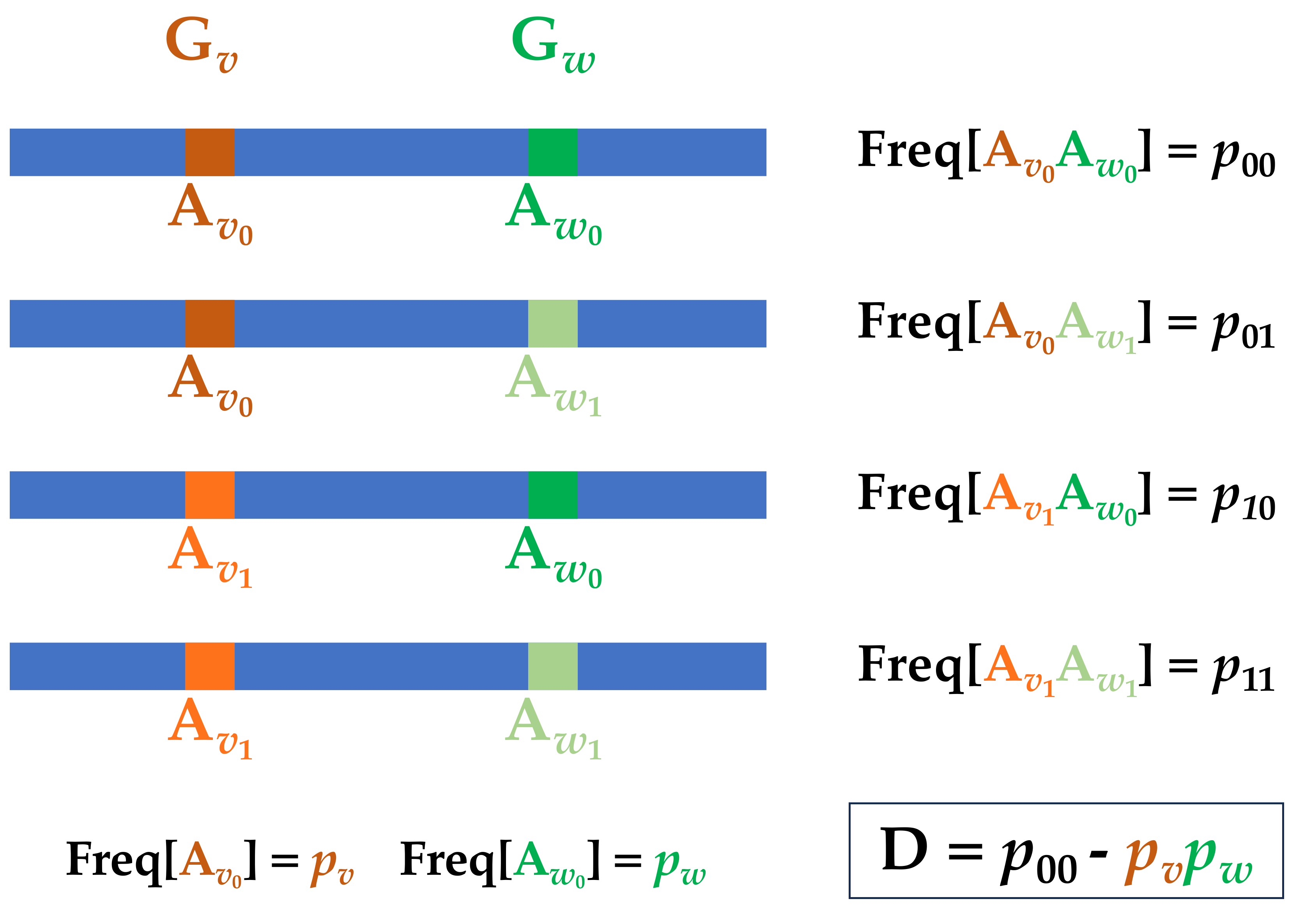
To begin to develop a framework for explicit accounting for LD, we start with some formal definitions. Imagine two genetic loci G_v and G_w with alleles $A_{v_{0}}, A_{v_{1}}$ and $A_{w_{0}}, A_{w_{1}}$ respectively. Let us further assume that these two genetic loci reside on the same chromosome. Thus, there are four possible haploid entities that population geneticists often call “gametes,” and human geneticists “haplotypes,” that represent the identity of all possible allelic combinations at these two loci on a single piece of DNA. Let p_v and p_w be the frequency of the $A_{v_{0}}$ allele and $A_{w_{0}}$ allele respectively. Let q_v = 1 – p_v, q_w = 1 – p_w be the frequency of the other allele at each locus. Let p₀₀, p₀₁, p₁₀, p₁₁ be the frequencies of a haplotypes containing the $A_{v_{0}} A_{w_{0}}, A_{v_{0}} A_{w_{1}}, A_{v_{1}} A_{w_{0}}, A_{v_{1}} A_{w_{1}}$ alleles respectively (Figure 1).

Figure 1 Two locus LD.

The population geneticist [6] defines, D, the standard measure of linkage disequilibrium, and the related r² as

\begin{array}{l} D & = & p_{00} - p_{v} p_{w} \\ = & - p_{10} + q_{v} p_{w} \\ = & - p_{01} + p_{v} q_{w} \\ = & p_{11} - q_{v} q_{w} \\ p_{v} & = & p_{00} + p_{01} . \\ q_{v} & = & p_{10} + p_{11} . \\ p_{w} & = & p_{00} + p_{10} . \\ q_{w} & = & p_{01} + p_{11} . \\ p_{00} & = & p_{v} p_{w} + D \\ p_{01} & = & p_{v} q_{w} - D \\ p_{10} & = & q_{v} p_{w} - D \\ p_{11} & = & q_{v} q_{w} + D \\ r^{2} & = & \frac{D^{2}}{p_{v} q_{v} p_{w} q_{w}} \end{array}

While this historical definition has its applications, a far more intuitively informative presentation begins by thinking of the alleles at G_v and G_w as Bernoulli random variables on {0, 1} with the state of Bernoulli variable determined by the state of the allele at the locus on a given haplotype. Thus, consider jointly distributed Bernoulli random variables B_v,B_w ∈{0, 1} to correspond to the state of the alleles at G_v and G_w on some randomly picked haplotype. With this in mind,

\begin{array}{l} E [B_{v}] & = & Pr [Picked A_{v_{0}}] \times 0 + Pr [Picked A_{v_{1}}] \times 1 \\ = & q_{v} . \\ E [B_{w}] & = & q_{w} . \\ Var [B_{v}] & = & E [B_{v}^{2}] - E {[B_{v}]}^{2} \\ = & Pr [Picked A_{v_{1}}] \times 1^{2} - q_{v}^{2} \\ = & q_{v} - q_{v}^{2} = p_{v} q_{v} . \\ Var [B_{w}] & = & p_{w} q_{w} . \\ Cov [B_{v}, B_{w}] & = & E [B_{v} B_{w}] - E [B_{v}] E [B_{w}] \\ = & Pr [Picked A_{v_{1}} A_{w_{1}}] \times 1 - q_{v} q_{w} \\ = & p_{11} - q_{v} q_{w} \\ = & D . \\ r^{2} & = & \frac{{(C o v [B_{v}, B_{w}])}^{2}}{Var [B_{v}] Var [B_{w}]} . \end{array}

Thus, the classical population genetics measure of LD, D, is nothing more than what might be called the haplotypic covariance, and the LD measure r² is the squared correlation coefficient between the alleles at the two loci. Higher order LD can be expressed in terms of higher order covariance terms.

To form an intuition for how this effects quantitative genetics quantities, let us assume there is no dominance at either locus, and that the only interaction between these two loci is induced by LD. Thus, let us begin by generalizing our notion of α, the average phenotype of an individual with a randomly picked allele, to η the average phenotype of an individual given a randomly picked haplotype. Letting H donate a haplotype randomly picked from an individual in this population,

\begin{array}{l} η_{v_{i}, w_{k}} & = & E [P | H = A_{v_{i}} A_{w_{k}}] \\ = & \sum_{j l} p_{j l} γ_{v_{i j}, w_{k l}} . \end{array}

If we assume there are no interactions between these loci other than that which is induced by LD, then $η_{v_{1}, w_{1}} - η_{v_{1}, w_{0}} = η_{v_{0}, w_{1}} - η_{v_{0}, w_{0}}$ and $η_{v_{1}, w_{0}} - η_{v_{0}, w_{0}} = η_{v_{1}, w_{1}} - η_{v_{0}, w_{1}}$ , In other words, the lack of interaction other than LD implies the difference in average phenotype between the alleles at the second locus are unaffected by the state of the first locus, and vice versa. The only interaction here is caused by the correlation in allelic state induced by LD. If a randomly picked individual has phenotype P with genotype $G_{v} = A_{v_{i}} A_{v_{j}} G_{w} = A_{w_{k}} A_{w_{l}}$ with corresponding haplotypes $A_{v_{i}} A_{w_{k}}$ and $A_{v_{j}} A_{w_{l}}$ then

\begin{array}{l} α_{v_{0}} & = & \frac{p_{00} η_{v_{0}, w_{0}} + p_{01} η_{v_{0}, w_{1}}}{p_{v}} . \\ α_{w_{1}} & = & \frac{p_{10} η_{v_{1}, w_{0}} + p_{11} η_{w_{1}, w_{1}}}{q_{v}} . \\ β_{v} & = & α_{v_{1}} - α_{v_{1}} \\ = & \frac{p_{v} p_{10} η_{v_{1}, w_{0}} - q_{v} p_{00} η_{v_{0}, w_{0}} + p_{v} p_{11} η_{v_{1}, w_{1}} - q_{v} p_{01} η_{v_{0}, w_{1}}}{p_{v} q_{v}} \\ = & \frac{p_{v} (q_{v} p_{w} - D) η_{v_{1}, w_{0}} - q_{1} (p_{v} p_{w} + D) η_{v_{0}, w_{0}}}{p_{v} q_{v}} \\ + \frac{p_{v} (q_{v} q_{w} + D) η_{v_{1}, w_{1}} - q_{v} (p_{v} q_{w} - D) η_{v_{0}, w_{1}}}{p_{v} q_{v}} \\ = & [p_{w} (η_{v_{1}, w_{0}} - η_{v_{0}, w_{0}}) + q_{w} (η_{v_{1}, w_{1}} - η_{v_{0}, w_{1}})] \\ + (\frac{D}{p_{v} q_{v}}) [p_{v} (η_{v_{1}, w_{1}} - η_{v_{1}, w_{0}}) + q_{v} (η_{v_{0}, w_{1}} - η_{v_{0}, w_{0}})] \\ = & [p_{w} (η_{v_{1}, w_{0}} - η_{v_{0}, w_{0}}) + q_{w} (η_{v_{1}, w_{1}} - η_{v_{0}, w_{1}})] \\ + (\frac{D}{p_{v} q_{v}}) [p_{v} (η_{v_{0}, w_{1}} - η_{v_{0}, w_{0}}) + q_{v} (η_{v_{1}, w_{1}} - η_{v_{1}, w_{0}})] \\ α_{w_{0}} & = & \frac{p_{00} η_{v_{0}, w_{0}} + p_{10} η_{v_{1}, w_{0}}}{p_{w}} \\ α_{w_{1}} & = & \frac{p_{01} η_{v_{0}, w_{1}} + p_{11} η_{v_{1}, w_{1}}}{q_{w}} \\ β_{w} & = & α_{w_{1}} - α_{w_{0}} \\ = & [p_{v} (η_{v_{0}, w_{1}} - η_{v_{0}, w_{0}}) + q_{v} (η_{v_{1}, w_{1}} - η_{v_{1}, w_{0}})] \\ + (\frac{D}{p_{w} q_{w}}) [p_{w} (η_{v_{1}, w_{0}} - η_{v_{0}, w_{0}}) + q_{w} (η_{v_{1}, w_{1}} - η_{v_{0}, w_{1}})] . \end{array}

With these results in mind, let us now imagine an idealized population that is identical to the current population in every way, except that there is no LD (D = 0) between these loci. Call the difference in allelic effect sizes (β_v and β_w in the actual population) $\tilde{β_{v}}$ and $\tilde{β_{w}}$ in the idealized population with no LD. >From the results above we immediately have

\begin{array}{l} \tilde{β_{v}} & = & [p_{w} (η_{v_{1}, w_{0}} - η_{v_{0}, w_{0}}) + q_{w} (η_{v_{1}, w_{1}} - η_{v_{0}, w_{1}})] . \\ \tilde{β_{w}} & = & [p_{v} (η_{v_{0}, w_{1}} - η_{v_{0}, w_{0}}) + q_{v} (η_{v_{1}, w_{1}} - η_{v_{1}, w_{0}})] . \\ β_{v} & = & \tilde{β_{v}} + \frac{D}{p_{v} q_{v}} \tilde{β_{w}} \\ β_{w} & = & \tilde{β_{w}} + \frac{D}{p_{w} q_{w}} \tilde{β_{v}} \end{array}

In this manner we arrive at the fundamental intuition concerning LD’s influence on effect sizes. The effect size at locus v, measured as the difference in average phenotype between individuals with an A₁ versus A₀ allele at locus v, is equal to what the effect size would be at locus v, absent LD, plus the effect at locus w, absent LD, weighted by the haplotypic covariance between the two loci, divided by the allelic variance at locus v, a quantity that might be called the “LD regression coefficient.” This is all formally true within our Kempthorne inspired interpretations of allelic effects. In a more Falconer inspired view, we would likely think of β̃_v and β̃_w as the “true” effect sizes at the two loci, with β_v and β_w being thought of as the “estimated” effects in the presence of LD. With a Falconer view in mind, we might phrase this most simply as the apparent effects at one SNP is the sum of the true effect at the SNP, plus the effects of another SNP times the LD regression coefficient between them. Whether one thinks of β̃ as either the “true” effect (in the Falconer sense) or the effect in a population absent LD (in the Kempthorne sense), calculation of β̃ could prove extremely useful in applications where effects estimated in one population will be applied to another population with differing LD. This also suggests a potential approach for accounting for LD in a study. If we again assume a lack of dominance or interaction from any source other than LD, and further assume that higher order LD is reasonably approximated by pairwise LD, for all SNPs in a given region, we can begin by estimating their effect sizes, in the Kempthorne sense, $\vec{β}$ . If we also have estimates of the LD covariance (D_v_,w) between all pairs of sites [v,w], and individual site allele frequencies p_v, q_v, we can construct an LD regression matrix M with $m_{v, w} = \frac{D_{v, w}}{p_{v} q_{v}}$ , and use the relationship

\begin{array}{l} \vec{β} & = & M \vec{\tilde{β}} . \\ \vec{\tilde{β}} & = & M^{- 1} \vec{β} . \end{array}

In practice, the LD matrix is likely to be very stiff (frequently with degenerate rows from pairs of sites in perfect LD), so there will necessarily be numerical challenges with implementing this sort of approach, but in principle this idea could be used for explicit accounting for LD, and application of estimates taken from one LD setting into another. Of course, this suggestion assumes the number of sites in LD with each other is small enough that a matrix inversion is plausible (i.e., thousands, not billions of sites). Population subdivision induces the appearance of LD between unlinked sites, i.e., haplotypic covariance between sites not actually on the same haplotype, throughout the entire genome, and as a result the number of sites in LD with one another can be, effectively, the entire genome when population subdivision is present. This is the fundamental reason estimation of effects generally include covariates measuring or accounting or population structure. This topic will be treated in much greater detail in the third paper in this series.

2.5 Intuition about distributions, interaction, and scaling

The only point in which normality of phenotype was assumed was when heritability was used to predict the mean phenotype of one relative given the other. Regardless of whether or not normality of phenotype holds, all of the quantities described here exist and are well defined. Defining narrow sense heritability as h² = V_A/V_P, heritability is well-defined and can be estimated from the covariance between relatives as described. Whether it has the property of predicting the phenotype of one relative given the other may depend on how closely the phenotypic distribution resembles a normal distribution, but heritability exists and is well-defined. In general, knowing the full distribution of the phenotype can be incredibly important because it can guide the choice of statistical model for inference, and choosing the wrong model often leads to unreliable estimation, inference, and prediction. These issues are seen again in the discussion of binary phenotypes below.

Nothing about this derivation assumed that factors are in any sense independent or interact in an additive fashion. Interactions are defined in terms of a deviation between observed conditional mean phenotype and the expected if the factors did happen to interact in an additive fashion. When additivity holds these interactions will be 0. Thus, assuming additivity is exactly equivalent to assuming that interactions do not exist, and vice versa. In a particularly important situation, LD, interactions between neighboring sites exist, and often result in a negative total interaction.

Overall we can view the total interactions as being contributed by two components. The first component is a variance induced by a deviation from additivity caused by the effect of two or more factors differing from the sum of the individual factor effects, e.g., $Var [d_{I g_{v, w}}]$ . This component will be positive whenever the combined effects of multiple factors does not equal the sum of their individual effects. The other component is induced by correlation between the states of the factors and are covariance terms. If the genotype at one locus is correlated with the genotype at another, if the genotype at a locus is correlated with an environmental state, or two environmental states are correlated with each other, these covariances could be non-zero, and might be negative. Thus, interactions can be thought of as composed of a variance contributed by a deviation from additivity, and covariances caused by non-independence of genotype, environment, or both. For uncorrelated genes / environments, all interactions are the variance due to deviation from additivity.

Nothing about this depends on phenotypes being normally distributed, or that the factors interact in an additive fashion, or that the factors are on similar “scales.” An interaction arises when factors have correlated states, or if the average phenotype of a combination of factors differs from the sum of their individual effects. Assuming a sufficiently large number of observations, for discrete factors such as genotype or those environments that can only take a finite number of different states, interactions can be estimated directly from individual-level data – data that gives phenotype and the factor states (such as genotype) for all individuals – essentially by finding one mean and subtracting another mean. This is all well-defined, above. If on the scale phenotype is measured, the effect of the combination of factors is the sum of the individual effects, no interaction exists. Otherwise it does. A non-linear transformation of the scale of the phenotype (taking the log of the phenotype, say) will necessarily change the size or even the existence of interactions. On one phenotypic scale, there might be no interactions, but on some other non-linear transformation, interactions may exist and be large. Thus, by definition, an interaction exists, or does not exist, on the scale on which the phenotype is measured. Change the scale, change the nature and size of the interaction. Interaction is not a biological quantity here, but a statistical one that describes the relationship of conditional expectations on whatever scale phenotype is measured. The strong law of large numbers convinces us that when phenotype is measured in a way that results in the phenotype being approximately normally distributed, we are likely to observe fewer statistical interactions. As a result it is often helpful to transform phenotypes to have a more normal like distribution, so that less of the total phenotypic variance derives from interaction. The partition of variance into their additive, dominance and interaction components is fundamentally, unavoidably, a function of the scale on which phenotype is measured. Change the scale in a non-linear way, and the partition of the variance components will change. Concepts of heritability are defined with respect to the scale of the phenotype. As quantitative geneticists we think of the scale which makes phenotype appear closest to normally distributed as the “natural scale” because this is the scale which usually results in the largest fraction of the variance being additive, and thus is the scale with the greatest power to predict one individual’s phenotype given a relative, which may be the goal of the analysis.

For continuously distributed factors there is a fundamental challenge not with definition, but with estimation. The interaction is still defined as the difference between the multivariate conditional expectation, and the sum of the marginal conditional expectations, but there is a central challenge involved with estimating those conditional expectations. Efficient estimation likely requires knowledge of the underlying multivariate distribution. For multivariate normal distributions with constant and equal variances, this value can be conveniently estimated as a cross-product term in a linear regression. For multivariate distributions with more complicated variance structures, interactions may be estimable more robustly in a general linear model framework, or with other even more sophisticated schemes. Nevertheless, the quantitative geneticist must never lose track of the fact that a cross-product term in some sort of linear model is not the definition of an interaction, but a method to estimate the interaction. When the underlying factors are continuous, this may be the only convenient method of estimation. In practice the utility of a cross-product estimator in a linear modeling framework will likely be deeply dependent on deviations from normality, the scale of the underlying factors, and covariance structures between the factors. Thus, for traits with a continuously large number of states, the efficiency of the interaction estimator may be crucially dependent on the scale of the phenotype and the scale of the underlying factors. For factors with only a finite number of states (like genotype), with a sufficiently large number of observations of the factors under consideration, interactions can always be estimated more simply as a difference in means. Problems associated with the estimation of interactions using a cross-product term in a linear model can be avoided for any discrete factor, such as genotypes or environments, with only a finite number of observable states.

2.6 Intuition about dominance and interaction sizes

Dominance is a term used by population geneticists to describe the relationship between the phenotype of the heterozygote and the two homozygotes. If the heterozygote has a phenotype equal (or nearly equal) to one of the homozygotes, we tend to say the allele associated with the homozygote genotype which is equal to the heterozygote phenotype is “dominant” to the other allele. Conversely we say the allele associated with other homozygote genotype is “recessive.” Additivity is a form of partial or incomplete dominance where heterozygote phenotype is between the two homozygous phenotypes. Over/Underdominance is used to describe heterozygote phenotypes outside the range of the two homozygotes (above/below).

These definitions are well ingrained in population genetics. Dominance is nearly synonymous with the phenotype of the heterozygote. As a result there is, perhaps, an intuitive desire to believe that a quantitative locus can be described as either additive, or if not additive with only one additional parameter to describe the heterozygous phenotype, ala 1, 1 – hs, 1 – s in a single locus population genetics scenario. This is simply not true when the additive effect is defined as the mean phenotype of the allele. A locus is either additive, in which case all three dominance deviations are 0, or it is not additive, in which case all 3 deviations are non-zero. Any attempt to parameterize this system with only two or fewer values will lead to none of them being interpretable as the additive effect, unless the locus is additive.

Another important insight is that the size of the dominance variance is very much a function of allele frequency. The only possible way for the dominance variance to be a large fraction of the total genetic variance is for the rare allele to be significantly recessive, i.e., for the heterozygote to have phenotype much closer to the common homozygote phenotype. This can be intuitive. Rare alleles are found more often as heterozygotes than homozygotes. The rarer the allele the truer this is. So, the mean phenotype of a rare recessive allele tends to be closer to the heterozygote phenotype than the homozygote, which results in greater deviation from additivity. Intuitively the additive approximation to all three genotype means is most in “error” when the rare allele is most recessive, and the size of this error increases with increasing rarity of the recessive allele. Stated the other way around, for a recessive locus where the recessive allele is common, most of the genetic variance will be additive. A recessive locus where the recessive allele is rare will have mostly dominance variance.

Finally it should be clear that each of the interaction terms is defined by the difference between the observed mean phenotype and what would be expected under additivity plus all the interactions at a “higher level”. Additive by dominance expectations include all the appropriate additive by additive interactions. Three way additive expectations include all the appropriate two-way (additive-by-additive) interactions, etc. Thus, unless there is a complicated pattern of correlation between states, it should be common for each level of interaction to be smaller in magnitude than the previous level. In the absence of correlation between states, each level of interaction is the residual variance after accounting for all the main and interaction effects on the previous level. As a result it is perfectly natural to expect V_G > V_GG > V_GGG > …..

3. Results and Discussion

Many human “disease” phenotypes, diastolic blood pressure, say, are well modeled and understood using the quantitative genetic machinery described above. Diastolic blood pressure is approximately normally distributed in most studies [14]. Investigators can and frequently do estimate heritability of the trait from family studies (sib-pairs or parents and offspring, say) [15] in the manner described above. At individual SNPs, the effect, β = α₁ – α₀, of substituting an A₁ allele for an A₀ is frequently estimated in some sort of regression framework. If we call this locus v, the heritability due to locus v, $h_{v}^{2}$ , can be estimated from this regression analysis [16]. Recalling as shown above pα₀ + qα₁ = 0,

\begin{array}{l} h_{v}^{2} & = & \frac{Var [a_{v}]}{V_{P}} . \\ Var [a_{v}] & = & 2 (p α_{0}^{2} + q α_{1}^{2}) \\ = & 2 (p α_{0}^{2} (p + q) + q α_{1}^{2} (p + q)) \\ = & 2 (p^{2} α_{0}^{2} + p q α_{0}^{2} + p q α_{1}^{2} + q^{2} α_{1}^{2}) \\ = & 2 (p^{2} α_{0} \frac{- q α_{1}}{p} + p q α_{0}^{2} + p q α_{1}^{2} + q^{2} α_{1} \frac{- p α_{0}}{q}) \\ = & 2 (- p q α_{0} α_{1} + p q α_{0}^{2} + p q α_{1}^{2} + - p q α_{0} α_{1}) \\ = & 2 p q (α_{0}^{2} - 2 α_{0} α_{1} + α_{1}^{2}) \\ = & 2 p q {(α_{1} - α_{0})}^{2} \\ = & 2 p q β^{2} . \end{array}

Thus, in a standardly designed Genome-Wide Association Study (GWAS) of a quantitative disease phenotype, such as diastolic blood pressure, the phenotype, P, is measured in a large number of individuals, and in those same individuals genotype is determined at a large (perhaps 10⁶ or more) number, n, of SNPs. At each locus the A₀ and A₁ alleles are coded as 0 and 1 respectively, and the genotype is coded as the sum of the alleles. The investigator then performs n independent linear regressions of phenotype as the outcome and genotype as the predictor, including any measured environmental co-variates that correlate with outcome, and often co-variates estimated from the entire genome’s genotypes to account for population structure within the study [17]. Alternatively, and perhaps more technically appropriate, a linear-mixed model might be performed where the rest of the genome’s genotype is treated as a random (≈ V_A) effect [18] . A detailed discussion of why these measures of genome-wide genotype are included is a topic of paper three.

The result of this study is n independently estimated β’s. If none of these sites were in LD with one another, and no other genetic interactions exist, and there are SNPs in all areas of the genome with genetic contributions to phenotype, V_A, and consequently heritability, could be estimated as 2pqβ² summed across all SNPs. This is the insight that lies at the heart of LD Score regression and related methods [19]. Alternatively, V_A could be estimated as the random effect term in a linear mixed model [20].

Somewhat recently, a frequently useful form of analysis has developed, often called polygenic risk scores (PRS) [21] or some related phrase. In this form of analysis, β’s are usually estimated in one study, and then in a second study, individuals with known genotype have their expected phenotype calculated using the first study’s β’s. Details and challenges associated with this style of analysis will be discussed in much greater detail in the second in this series of papers.

3.1 Binary traits

In many ways, the field of human genetics arose largely independently of any quantitative genetics ideas. For much of its early history [22, 23] the field was largely concerned with understanding nearly binary traits (traits with only two major phenotypes) under nearly Mendelian control (single locus genetics). At first glance, there was no obvious connection between the modeling framework presented here [24], which often results in approximately normally distributed phenotypes, and the approximately binary traits that were of deepest interest to human geneticists.

In a seminal 1965 work, Falconer [25] made clear a natural connection between human binary phenotypes and the quantitative genetics framework used here. The key idea was to suppose that a binary phenotype is like any other quantitative phenotype, but observed on “the wrong scale.” For any binary trait of interest, Crohn’s Disease (CD), say, humans are characterized as either having CD, or not. However, following Falconer, quantitative geneticists will think about CD like any other quantitative trait. To do so, they will assume there is a related trait which they will generally call “liability” to CD. This trait, liability to CD, is a quantitative trait like any other. It is contributed to by genes and the environment. Its variance components can be decomposed as described above. However, liability is not directly observable. One can not observe or measure liability to CD directly. Instead, the effects of the existence of a threshold t on that liability scale can be observed (Figure 2). Individuals with liability greater than or equal to t are observed to have CD. Individuals with liability less than t do not have CD.

Figure 2 Normally distributed liability with disease determining threshold at liability greater than 2.

In our personal experience, many physician scientists will immediately express skepticism about the applicability or utility of this abstraction, “liability to disease,” to their particular areas of study. Interestingly, one of the first implications of this abstraction is that there ought to exist individuals with liability very near the threshold. Presumably such individuals will often be very hard to classify. They are “unaffected” people who nearly have the disease, or they are affected people who have only a very mild form of the disease. These are individuals who two well trained physicians might reasonably disagree on whether or not such a person formally qualifies for diagnosis of the disease. Viewed in this light, we can see the abstraction of an unobservable liability is the cause of the existence of individuals who either slightly do, or do not, reach diagnostic criteria for a disease. Such individuals have liability very near the threshold, and because liability is unobservable directly, two perfectly well trained physicians may disagree about which side of the threshold a particular individual lies.

For all that follows we will treat this threshold on the liability scale as a fixed quantity determined inexorably by nature. As such, this threshold is very much a theoretician’s abstraction. The threshold exists, and therefore some people have disease and others do not. It offers nothing resembling insight or intuition for how and why it exists or how differing groups of people might have differing frequency of disease, other than to say their thresholds must differ. In the fourth paper in this series, the thresholding model will be examined in some detail with particular emphasis on understanding how prevalence differences between males and females can be understood and modeled, with a particular emphasis on examining the effect of the X-chromosome.

While we have gone to pains to emphasize that very little before this point made any assumption about the distribution of phenotype, because liability is unobserved, in order to make any further progress we must make some assumptions about the distribution of liability. Here we assume for the first time that liability is well approximated with a normal distribution. We are not assuming all factors are additive, or that correlation in states do not exist, but we are assuming that enough uncorrelated factors exist that some version of the strong-law of large numbers holds and that liability is nearly normally distributed [26]. While it is certain that many (most) observable traits are nearly normally distributed [27], the assumption of complete convergence in distribution to normality is a far stronger assumption than we have made up to this point. That meaningful departure from normality may not be particularly common even in the presence of linkage disequilibrium, some alleles of moderate effect, and strong selection (disease itself is likely a selective pressure) [28] is reassuring. Thus, here for the first time we assume a fully normally distributed trait, which we call liability to some binary phenotype, often a human disease. Because this normally distributed trait is unobserved, we can assume it is parameterized in anyway we please. For convenience we will assume that liability has mean 0, and total variance V_P = 1, i.e., follows a “standard” normal distribution. For such traits heritability h² = V_A/V_P = V_A. Thus, it will not be uncommon for human quantitative geneticists to call something heritability or a contribution to heritability, while clearly estimating V_A, or $V_{a_{v}}$ the additive variance due to locus v. In fact, as a field $V_{a_{v}}$ is often called the “SNP heritability” of locus v. When V_P = 1 heritability and additive variance are identical in value, but interchanging their terms can certainly lead to confusion, particularly in students new to the field. Finally, for convenience we will always orient the threshold t to be a positive value. Thus, by convention increasing liability increases the chance of disease, and decreasing liability has the opposite effect.

3.2 Human disease quantities

The human genetics field often has its own set of terms of art that are sometimes confusing to classically trained population or quantitative geneticists. Above we saw that human geneticists often call Wright’s IBD probabilities Cotterman coefficients. Here, for the sake of explicit understanding, we will define several terms that frequently occur in human disease studies.

We begin by assuming there is a population of humans that at least approximately corresponds to a single, finite Fisher-Wright population in Hardy-Weinberg equilibrium. In this population, there is a quantitative phenotype L, which is the liability to some disease of interest. There is a threshold, t, on this liability scale such that individuals with liability above this threshold, L > t, are said to be diseased, and individuals with liability below t are said to be “healthy” or not to have the disease in question. The term “prevalence” of a disease, ψ is the fraction of the population with disease and is uniquely determined by t,

\begin{array}{l} ψ & = & \int_{t}^{\infty} ϕ (x) d x \\ = & 1 - Φ (t) \\ t & = & Φ^{- 1} (1 - ψ), \end{array}

where ϕ(x) is a standard normal probability density, Φ(x) is a standard normal cumulative distribution, and Φ^–1(x) is its inverse. Thus, we think of the prevalence of a disease as determining the threshold on the liability scale beyond which individuals are diseased.

It might be noted throughout everything that we have done, we have ignored an important practical consideration. Many, perhaps most, phenotypes change over the course of an organism’s lifetime. Weight, height, blood pressure, can change as an individual gets older. Thus, from a practical standpoint phenotype might have been defined and measured relative to some age, weight at age 10 years, or blood pressure at age 50-60, say. Alternatively, we might ignore this issue entirely and allow the phenotypic measure to include anyone at any age, and therefore if the phenotype varies over age, some of the phenotypic variance is likely accounted for by age itself. In this context age is best viewed as an environmental factor contributing to phenotype. With respect to a binary phenotype, we see these concepts played out in notions of “incidence” and “prevalence.” Like seemingly all terms in genetics, there is variability in how these terms are used and defined, but often incidence is used as a measure of the number of individuals who newly develop a binary phenotype within a short period of time. Prevalence is usually used as the sum of incidence over a period of interest. Thus, you can think of the incidence as the rate disease is diagnosed, and prevalence as the total fraction of diseased individuals diagnosed during that time. When very precisely defined, incidence might be a density and prevalence a cumulative distribution. Prevalence, therefore, likely includes some measure of age in its definition (disease before age 21, say), or if anyone at any age is included, prevalence is best thought of as “lifetime” prevalence, the fraction of individuals diagnosed with the condition at any point before death. Here we use prevalence to mean the total fraction of the population with the disease, however that population is defined with respect to age.

One of the key questions in human genetics is “What effect does a given SNP have on disease liability?” Within our Kempthorne framework, we imagine this effect causes the mean liability of individuals with different genotypes to differ (Figure 3). If we could observe liability directly, we could immediately apply all of the previous machinery. Here, though, liability is not directly observed. Instead, in the classical human genetics experiment, a number N_D people with disease are identified along with $N_{D}$ people without the disease. By convention people with the disease are often called “cases” and people without the disease called “controls.” Cases and controls are often collected in a very biased way relative to disease prevalence. Usually cases are dramatically oversampled such that $N_{D} ≫ ψ N_{D}$ . Regardless of the sampling proportions, the fundamental data collected is the counts n₀₀,n₀₁,n₁₁ of the three genotypes A₀A₀, A₀A₁, A₁A₁, broken down by case, $n_{i j}^{D}$ , and control $n_{i j}^{D}, n_{i j} = n_{i j}^{D} + n_{i j}^{D}$ status. It is perhaps not immediately intuitive, but given disease prevalence ψ, these counts are sufficient to estimate all of the above described quantitative genetics quantities. If f_ij and allele p, q are the true genotype and allele frequencies in the population, and $f_{i j}^{D}, f_{i j}^{D}$ corresponding values in the diseased and not diseased subsets of the population, we can begin by estimating $\hat{f_{i j}^{D}}$ and $\hat{f_{i j}^{D}}$ from case / control count data, and then proceed using these estimates in place of the parameters they represent.

Figure 3 Genotypes with differing mean liability have differing penetrances. Each genotype’s liability density has equal variance, 1 – V_g, but unequal means. p = 0.7, γ₁₁ = 0.5, γ₀₁ = 0.1. In the top panel, the area under each liability curve is scaled to the genotype frequency, p², 2pq, and q².

\begin{array}{l} \hat{f_{i j}^{D}} & = & \frac{n_{i j}^{D}}{N_{D}} \\ \hat{f_{i j}^{D}} & = & \frac{n_{i j}^{D}}{N_{D}} \\ p^{D} & = & f_{00}^{D} + \frac{f_{01}^{D}}{2} \\ q^{D} & = & 1 - p^{D} \\ p^{D} & = & f_{00}^{D} + \frac{f_{01}^{D}}{2} \\ q^{D} & = & 1 - p^{D} \\ f_{i j} & = & ψ f_{i j}^{D} + (1 - ψ) f_{i j}^{D} \\ p & = & ψ p^{D} + (1 - ψ) p^{D} \\ q & = & 1 - p . \end{array}

The term penetrance of X is the conditional probability of an individual being diseased given they are in state X. Thus, we can consider the penetrance ζ of a genotype G_ij, the probability an individual is diseased given their genotype is A_iA_j at this locus. We can also think about penetrance of an allele A_i, the probability an individual is diseased given they have an A_i allele. Thus,

\begin{array}{l} ζ_{G_{i j}} & = & Pr [L > t | G = A_{i} A_{j}] \\ = & Pr [D | G = A_{i} A_{j}] \\ ζ_{A_{i}} & = & Pr [L > t | A = A_{i}] \\ = & Pr [D | A = A_{i}] . \end{array}

With application of Bayes’ theorem, penetrances can be immediately estimated from the case/control data.

\begin{array}{l} Pr [D \cap G = A_{i} A_{j}] & = & Pr [G = A_{i} A_{j} | D] Pr [D] \\ = & Pr [D | G = A_{i} A_{j}] Pr [G = A_{i} A_{j}] . \\ ζ_{G_{i j}} & = & \frac{f_{i j}^{D} ψ}{f_{i j}} \\ ζ_{A_{0}} & = & \frac{p^{D} ψ}{p} \\ ζ_{A_{1}} & = & \frac{q^{D} ψ}{q} \end{array}

Thus, from the overall prevalence and genotype counts in cases and controls, we can estimate the penetrance (probability of disease given genotype/allele) of both alleles and all three genotypes. Of course, as quantitative geneticists we measure effect sizes in terms of mean effects on liability, but that too is now immediately available, with a sensible approximation, or can be found numerically. To find this, recall that we have normalized liability to have V_P = 1. If the three genotypes at this locus have mean liability γ₀₀, γ₀₁, and γ₁₁ respectively, then

\begin{array}{l} V_{g} & = & f_{00} γ_{00}^{2} + f_{10} γ_{01}^{2} + f_{11} γ_{11}^{2} . \\ ζ_{G_{i j}} & = & \int_{t}^{\infty} ϕ (x; γ_{i j}, 1 - V_{g}) d x \\ = & \int_{t - γ_{i j}}^{\infty} ϕ (x; 0, 1 - V_{g}) d x \\ \approx & \int_{t - γ_{i j}}^{\infty} ϕ (x; 0, 1) d x . \\ γ_{i j} & \approx & t - Φ^{- 1} (1 - ζ_{G_{i j}}) . \\ α_{i} & \approx & t - Φ^{- 1} (1 - ζ_{A_{i}}), \end{array}

where ϕ(x; μ, σ²) is a normal density with mean μ and variance σ². The above approximations hold whenever V_g ≪ 1. Since for the vast majority of human disease [29] there are at most a handful of sites that explain more than 0.1% of the variance, this approximation is almost always very good. When trying to estimate something that explains a truly substantial fraction of the variance, a Newton-Raphson iteration (or just about any other kind of numerical search) will converge quickly. Nevertheless, even for very small genetic variances it is often useful to estimate “all but one” of the effects, and find the remaining effect using the fact that the average effect must be zero. Thus, it is often helpful to estimate these effects as

\begin{array}{l} γ_{11} & = & t - Φ^{- 1} (1 - ζ_{G_{11}}) . \\ γ_{01} & = & t - Φ^{- 1} (1 - ζ_{G_{01}}) . \\ γ_{00} & = & \frac{- (f_{11} γ_{11} + f_{01} γ_{01})}{f_{00}} . \\ α_{1} & = & t - Φ^{- 1} (1 - ζ_{A_{1}}) . \\ α_{0} & = & \frac{- q α_{1}}{p} \end{array}

Calculating effects in this manner assures that the population mean remains 0 despite the approximation used for the residual variance. Thus, starting with only prevalence and the counts of genotypes we have arrived at all the quantitative genetic quantities needed to calculate additive and dominance contributions to variance.

As discussed above, for quantitative traits, many researchers estimate interaction effects from a cross-product term in some sort of linear model. These estimation procedures tend to be most efficient when the underlying traits are normally distribtued. Since liability can not be directly observed, interactions can not be estimated in this fashion here. Nevertheless, higher order interactions can be approached the same way main effects are, via counts of individuals with two (or more) locus genotypes, divided between cases and controls. For instance, if $f_{v_{i j}, w_{k l}}^{D}$ and $f_{v_{i j}, w_{k l}}^{D}$ are the frequency of the combination of genotypes $A_{v_{i}} A_{v_{j}}$ and $A_{w_{k}} A_{w_{l}}$ at loci v and w, then

\begin{array}{l} f_{v_{i j}, w_{k l}} & = & ψ f_{v_{i j}, w_{k l}}^{D} + (1 - ψ) f_{v_{i j}, w_{k l}}^{D} . \\ ζ_{G_{v_{i j}, w_{k l}}} & = & \frac{f_{v_{i j}, w_{k l}}^{D} ψ}{f_{v_{i j}, w_{k l}}} . \\ γ_{v_{i j}, w_{k l}} & \approx & t - Φ^{- 1} (1 - ζ_{G_{v_{i j}, w_{k l}}}) . \\ δ_{I g_{v_{i j}, w_{k l}}} & = & γ_{v_{i j}, w_{k l}} - (γ_{v_{i j}} + γ_{w_{k l}}), \end{array}

and in a similar manner all other interaction quantities can be estimated. As discussed above, for continuously distributed factors, it may be impossible to estimate interaction on an unobserved liability scale, but for discrete factors such as genotype, interaction deviations and variances can be calculated directly from the difference between average liability for the combination of factors and the sum of the individual factor effects given only case/control frequencies and the assumption of an approximately normally distributed liability.

Historically effect sizes in human genetics tend to be reported as either a “relative risk” or an “odds ratio.” Both quantities are some sort ratio of the penetrances. In general, the relative risk of X to Y, is $\frac{Pr [D | X]}{Pr [D | Y]}$ , i.e., it is the ratio of the penetrance of X to the penetrance of Y. Building on historical gambling terms, the “odds” of something is the probability the event happens, divided by the probability the event does not happens. Thus the odds of X are $\frac{Pr [D | X]}{1 - Pr [D | X]}$ . So, the odds ratio of X to Y is $\frac{Pr [D | X] (1 - Pr [D | Y])}{Pr [D | Y] (1 - Pr [D | X])}$ . Thus, it might be natural to discuss the odds ratio of the A₁ allele to the A₀ allele, or even the G₁₁ genotype to the G₀₀ genotype, say.

For very practical reasons the odds ratio of A₁ to A₀ (or the other way around) is the most commonly reported effect size estimate in all human genetics studies. The reason for this is that odds ratios (OR) can be estimated in the presence of covariates in a very natural way. Recall for a classically observed quantitative phenotype we might commonly estimate β for a SNP from a linear regression (or linear mixed model, etc.) that included any covariates known to correlate with phenotype, such as some measured environmental variable (or related quantity such as sex or age), and almost always including estimates of genome-wide genotype to account for population structure (the fact that not all samples come from a single idealized randomly mating population). The outcome of this linear regression is an estimate of the mean effect β of substituting an A₁ allele for an A₀ allele on phenotype. From strictly genotype count data it is hard to immediately imagine a framework that would allow estimation of β while accounting for covariates in a similar fashion. Logistic regression turns out to be the non-obvious, but extremely practically useful approach to the problem.

To understand why, Figure 4 plots the penetrance on the Y-axis of an allele with mean liability (Z, shown in standard deviations where a standard deviation is $\frac{4}{\sqrt{2 π}})$ on the X-axis for a trait with prevalence 0.5 and threshold t = 0 versus a standard logistic curve ( $\frac{1}{1 + e^{- x}}$ ). While this is for a very specific normal distribution, the intuition formed is that if liability is well approximated by a normal distribution then the penetrance for an allele is likely well approximated by a logistic function. Logistic regression is a relatively simple and widely available numerical procedure to estimate the odds ratio of A₁ to A₀ from case/control count data by fitting the observations to logistic curves for the penetrances of each allele. This is done without having to know prevalence, or even overall allele frequency, and the estimate can account for the effects of any number of covariates as simply as ordinary linear regression. The practicality and the utility of this approach should be clear.

Figure 4 Penetrance assuming normally distributed liability versus logistic approximation for a trait with threshold at 0.

To a quantitative geneticist the output of a logistic regression (the odds ratio OR) is not particularly useful per se. Absent knowledge of the disease prevalence, it can only be viewed as an approximation to an interesting but not particularly interpretable quantity. However, if disease prevalence is known (or estimated) the odds ratio can be converted into our standard measures of effect. To do so we note that

\begin{array}{l} Pr [D] & = & Pr [D | A_{0}] Pr [A_{0}] + Pr [D | A_{1}] Pr [A_{1}] . \\ ψ & = & p ζ_{A_{0}} + q ζ_{A_{1}} . \\ ζ_{A_{0}} & = & \frac{ψ - q ζ_{A_{1}}}{1 - q} . \\ OR & = & \frac{ζ_{A_{1}} (1 - ζ_{A_{0}})}{ζ_{A_{0}} (1 - ζ_{A_{1}})} . \end{array}

From the above one can solve for $ζ_{A_{0}}$ , albeit in a painful blizzard of algebra involving quadratic terms. Usually one assumes that the common allele has a penetrance nearly equal to population prevalence and reaches

\begin{array}{l} OR & \approx & \frac{ζ_{A_{1}} (1 - ψ)}{ψ (1 - ζ_{A_{1}})} \\ ζ_{A_{1}} & \approx & \frac{OR ψ}{1 + ψ (OR - 1)} \\ ζ_{A_{0}} & = & \frac{ψ - q ζ_{A_{1}}}{1 - q} . \end{array}

Of course, one could numerically iterate these ζ’s to converge to the exactly estimated OR, but given that the logistic curve itself is an approximation to penetrance of a normally distributed liability, seeking such precision seems a bit like overkill. Estimated in this fashion the two allelic penetrances are consistent with the overall prevalence of the disease, and for anything other than absurdly large effect sizes, have odds ratio close to the estimated value from the logistic regression. With the estimates of penetrances in hand, we can convert back to mean effects on the liability scale, and again use all of our standard quantitative genetics ideas to arrive at notions such as SNP heritability etc. estimated from a logistic regression with case/control counts.

3.3 Heritability of a disease

As first discussed by Falconer [25], this same framework allows us to estimate overall heritability of any binary phenotype such as a human disease. To do so, one first needs an estimate of disease prevalence ψ, and the disease threshold t, found as described above. Interestingly, and perhaps not instantly obvious, the disease threshold allows calculation of the average liability, E[L|D], of affected individuals.

\begin{array}{l} E [L | D] & = & \int_{t}^{\infty} x ϕ (x) d x \\ = & \frac{ϕ (t)}{ψ} . \end{array}

Thus, the mean liability of affected individuals is determined by the prevalence of disease. To this one adds data on affected pairs of individuals with a known familial relationship, for instance, pairs of siblings both affected with the disease, or a parent and offspring both affected, etc. The basic design is to first identify individuals with the disease. Such an individual is often called the “proband.” Identification of probands, being predicated on disease state, is necessarily biased relative to overall disease prevalence, but is assumed to be an unbiased collection of diseased individuals. Thus, probands are assumed to have average liability, E[L|D], as given above. Once identified, relatives of specific relatedness ρ to the proband are then identified as completely as possible, and the affectation status of these relatives is ascertained. For instance, the relatives might be a parent of the proband such that ρ = 0.5. The faction of these relatives ζ_relative who are also affected with disease is estimated. This fraction, ζ_relative, is an estimate of the penetrance of disease given the individual is the specified degree of relatedness to the proband. Thus, ζ_relative = Pr[D|relative], and we can find the mean liability of these relatives E[L|relative] with

E [L | relative] = t - Φ^{- 1} (1 - ζ_{relative}) .

In this manner we now have the mean phenotype of pairs of relatives with known relatedness ρ. We can then estimate disease heritability h² in the “usual” manner,

h^{2} = \frac{E [L | relative]}{ρ E [L | D]} .

4. Conclusions

Standard quantitative genetics quantities and results are derived from a first principles approach. Measures of a factor’s (gene, allele, or environment) effect size are defined as conditional expectation of phenotype given that factor. Main effects and interaction effects are defined with very limited assumptions. Linkage-disequilibrium’s contribution to effect size is derived, and methods to account for it are discussed. Application of this framework to binary traits, such as human disease, are extended with one additional assumption, that disease liability is well approximated by a normal distribution. Methods to calculate quantitative genetics quantities are demonstrated using case-control count data.

Declarations

Ethics Statement

Not applicable.

Consent for Publication

Not applicable.

Availability of Data and Material

Not applicable.

Funding

This study was supported by NIH Grant: RF1 AG071170.

Competing Interests

David J. Cutler is a member of the Editorial Board of the journal Human Population Genetics and Genomics. The author was not involved in the journal’s review of or decisions related to this manuscript. The authors have declared that no other competing interests exist.

Author Contributions

All authors participated in the derivation, writing, and editing of this work.

Acknowledgement

Population geneticists of a certain age will, without doubt, recognize the voice and influence of John H. Gillespie throughout this presentation. While attributed here to Kempthorne, because that is how he attributed it, it is certain that nearly the entirety of the methods section has at least transiently appeared on a blackboard 12 inches in front of a chalk covered Michael Turelli, feverishly deriving the next result with his right hand while erasing older results with his left.

Table 1 Summary of key variables.

Symbol	Description	Formalism
$A_{v_{0}}$	The major allele at locus v	$Freq [A_{v_{0}}] \geq Freq [A_{v_{1}}]$
$A_{v_{1}}$	The minor allele at locus v	$Freq [A_{v_{1}}] \leq Freq [A_{v_{0}}]$
p_v	Frequency of $A_{v_{0}}$	$p_{v} = Freq [A_{v_{0}}]$
q_v	Frequency of $A_{v_{1}}$	q_v = 1 – p_v
A_v	Random allele at locus v, $A_{v} \in {A_{v_{0}}, A_{v_{1}}}$	$Pr [A_{v} = A_{v_{0}}] = p_{v}, Pr [A_{v} = A_{v_{1}}] = q_{v}$
G_v	Random genotype at locus v, $G_{v} \in {A_{v_{0}} A_{v_{0}}, A_{v_{0}} A_{v_{1}}, A_{v_{1}} A_{v_{1}}}$	$Pr [G_{v} = A_{v_{0}} A_{v_{0}}] = p_{v}^{2}, Pr [G_{v} = A_{v_{0}} A_{v_{1}}] = 2 p_{v} q_{v}$ $Pr [G_{v} = A_{v_{1}} A_{v 1}] = q_{v}^{2}$
$γ_{v_{00}}$	Genotypic effect of $A_{v_{0}} A_{v_{0}}$	$γ_{v_{00}} = E [P \| G_{v} = A_{v_{0}} A_{v_{0}}]$
$γ_{v_{01}}$	Genotypic effect of $A_{v_{0}} A_{v_{1}}$	$γ_{v_{01}} = E [P \| G_{v} = A_{v_{0}} A_{v_{1}}]$
$γ_{v_{11}}$	Genotypic effect of $A_{v_{1}} A_{v_{1}}$	$γ_{v_{11}} = E [P \| G_{v} = A_{v_{1}} A_{v_{1}}]$
$α_{v_{0}}$	Allelic effect of $A_{v_{0}}$	$α_{v_{0}} = E [P \| A_{v} = A_{v_{0}}]$
$α_{v_{1}}$	Allelic effect of $A_{v_{1}}$	$α_{v_{1}} = E [P \| A_{v} = A_{v_{1}}] = \frac{- p_{v} α_{v_{0}}}{q_{v}}$
$β_{v}$	Difference in allelic effects	$β_{v} = α_{v_{1}} - α_{v_{0}}$
$δ_{v_{00}}$	Dominance deviation of genotype $A_{v_{0}}$ $A_{v_{0}}$	$δ_{v_{00}} = γ_{v_{00}} - 2 α_{0}$
$δ_{v_{01}}$	Dominance deviation of genotype $A_{v_{0}}$ $A_{v_{1}}$	$δ_{v_{01}} = γ_{v_{01}} - (α_{0} + α_{1})$
$δ_{v_{11}}$	Dominance deviation of genotype $A_{v_{1}}$ $A_{v_{1}}$	$δ_{v_{11}} = γ_{v_{11}} - 2 α_{1}$
g_v	Random genetic effect determined by G_v	If $G_{v} = A_{v_{i}} A_{v_{j}}$ , then $g_{v} = γ_{v_{i j}}$
a_v	Random additive effect determined by G_v	If $G_{v} = A_{v_{i}} A_{v_{j}}$ , then $a_{v} = α_{v_{i}} + α_{v_{j}}$
d_v	Random dominance deviation determined by G_v	If $G_{v} = A_{v_{i}} A_{v_{j}}$ , then $d_{v} = δ_{v_{i j}}$
$V_{g_{v}}$	Total genetic variance of locus v	$V_{g_{v}} = p_{v}^{2} {(γ_{v_{00}})}^{2} + 2 p_{v} q_{v} {(γ_{v_{01}})}^{2} + q_{v}^{2} {(γ_{v_{11}})}^{2}$
$V_{a_{v}}$	Additive variance of locus v	$V_{a_{v}} = 2 (p_{v} α_{v_{0}}^{2} + q_{v} α_{v_{1}}^{2})$
$V_{d_{v}}$	Dominance variance of locus v	$V_{d_{v}} = p_{v}^{2} {(δ_{v_{00}})}^{2} + 2 p_{v} q_{v} {(δ_{v_{01}})}^{2} + q_{v}^{2} {(δ_{v_{11}})}^{2}$
$γ_{v_{00}, w_{00}}$	Genotypic effect of $A_{v_{0}}$ $A_{v_{0}}$ and $A_{w_{0}} A_{w_{0}}$	$γ_{v_{00}, w_{00}} = E [P \| G_{v} = A_{v_{0}} A_{v_{0}}, G_{w} = A_{w_{0}} A_{w_{0}}]$
$γ_{v_{00}, w_{01}}$	Genotypic effect of $A_{v_{0}}$ $A_{v_{0}}$ and $A_{w_{0}} A_{w_{1}}$	$γ_{v_{00}, w_{01}} = E [P \| G_{v} = A_{v_{0}} A_{v_{0}}, G_{w} = A_{w_{0}} A_{w_{1}}]$
$γ_{v_{00}, w_{11}}$	Genotypic effect of $A_{v_{0}}$ $A_{v_{0}}$ and $A_{w_{1}} A_{w_{1}}$	$γ_{v_{00}, w_{11}} = E [P \| G_{v} = A_{v_{0}} A_{v_{0}}, G_{w} = A_{w_{1}} A_{w_{1}}]$
$γ_{v_{01}, w_{00}}$	Genotypic effect of $A_{v_{0}}$ $A_{v_{0}}$ and $A_{w_{0}} A_{w_{0}}$	$γ_{v_{01}, w_{00}} = E [P \| G_{v} = A_{v_{0}} A_{v_{1}}, G_{w} = A_{w_{0}} A_{w_{0}}]$
$γ_{v_{01}, w_{01}}$	Genotypic effect of $A_{v_{0}}$ $A_{v_{1}}$ and $A_{w_{0}} A_{w_{1}}$	$γ_{v_{01}, w_{01}} = E [P \| G_{v} = A_{v_{0}} A_{v_{1}}, G_{w} = A_{w_{0}} A_{w_{1}}]$
$γ_{v_{01}, w_{11}}$	Genotypic effect of $A_{v_{0}}$ $A_{v_{1}}$ and $A_{w_{1}} A_{w_{1}}$	$γ_{v_{01}, w_{11}} = E [P \| G_{v} = A_{v_{0}} A_{v_{1}}, G_{w} = A_{w_{1}} A_{w_{1}}]$
$γ_{v_{11}, w_{00}}$	Genotypic effect of $A_{v_{1}}$ $A_{v_{1}}$ and $A_{w_{0}} A_{w_{0}}$	$γ_{v_{11}, w_{00}} = E [P \| G_{v} = A_{v_{1}} A_{v_{1}}, G_{w} = A_{w_{0}} A_{w_{0}}]$
$γ_{v_{11}, w_{01}}$	Genotypic effect of $A_{v_{1}}$ $A_{v_{1}}$ and $A_{w_{0}} A_{w_{1}}$	$γ_{v_{11}, w_{01}} = E [P \| G_{v} = A_{v_{1}} A_{v_{1}}, G_{w} = A_{w_{0}} A_{w_{1}}]$
$γ_{v_{11}, w_{11}}$	Genotypic effect of $A_{v_{1}}$ $A_{v_{1}}$ and $A_{w_{1}} A_{w_{1}}$	$γ_{v_{11}, w_{11}} = E [P \| G_{v} = A_{v_{1}} A_{v_{1}}, G_{w} = A_{w_{1}} A_{w_{1}}]$
g_v_,w	Random two locus genetic effect determined by genotypes G_v and G_w	If $G_{v} = A_{v_{i}} A_{v_{j}}, G_{w} = A_{w_{k}} A_{w_{l}}$ then $g_{v, w} = γ_{v_{i j}, w_{k l}}$
$δ_{I g_{v_{i j}, w_{k l}}}$	Epistatic Deviation	$δ_{I g_{v_{i j}, w_{k l}}} = γ_{v_{i j}, w_{k l}} - (γ_{v_{i j}} + γ_{w_{k l}})$
$δ_{I a a_{v_{i}, w_{k}}}$	Additive by Additive Deviation	$δ_{I a a_{v_{i}, w_{k}}} = E [P \| A_{v} = A_{v_{i}}, A_{w} = A_{w_{k}}] - (α_{v_{i}} + α_{w_{k}})$
$δ_{I a d_{v_{i}, w_{k l}}}$	Additive by Dominance Deviation	$δ_{I a d_{v_{i}, w_{k l}}} = E [P \| A_{v} = A_{v_{i}}, G_{w} = A_{w_{k}} A_{w_{l}}]$ $- (α_{v_{i}} + α_{w_{k}} + α_{w_{l}} + δ_{w_{k l}})$
$δ_{I d d_{v_{i j}, w_{k l}}}$	Dominance by Dominance Deviation	$δ_{I d d_{v_{i j}, w_{k l}}} = E [P \| G_{v} = A_{v_{i}} A_{v_{j}}, G_{w} = A_{w_{k}} A_{w_{l}}]$ $- (α_{v_{i}} + α_{v_{j}} + δ_{v_{i j}} + α_{w_{k}} + α_{w_{l}} + δ_{w_{k l}})$
L	An unobserved phenotype, liability to disease	L ~ Φ(x)
t	A threshold on the liability scale determining disease	Individual is diseased if L > t
ψ	Prevalence of the disease with liability L	$ψ = \int_{t}^{\infty} ϕ (x) d x$
ζ_y	The penetrance of some factor y	ζ_y = Pr[L > t\|y]

References

1.	Fisher RA. The Correlation between Relatives on the Supposition of Mendelian Inheritance. Trans Roy Soc Edinburgh 1918;52:399-433. [Google Scholar] [CrossRef]

2.	Moran PAP, Smith CAB, Fisher RA. Commentary on R.A. Fisher’s paper on the correlation between relatives on the supposition of Mendelian inheritance (Published for the Galton Laboratory, University College London). London: Cambridge University Press; 1966.

3.	Box JF. R. A. Fisher, the life of a scientist. New York: Wiley; 1978.

4.	Falconer DS. Introduction to quantitative genetics. Harlow, Essex, England: Longman, Scientific and Technical, Burnt Mill; New York: Wiley; 1989.

5.	Lynch M, Walsh B. Genetics and analysis of quantitative traits. Sunderland, MA: Sinauer; 1998.

6.	Gillespie JH. Population genetics: a concise guide. Baltimore, MD: Johns Hopkins University Press; 2004.

7.	Kempthorne O. The Theoretical Values of Correlations between Relatives in Random Mating Populations. Genetics 1955;40:153-67. [Google Scholar] [CrossRef]

8.	Jacob F, Monod J. Genetic regulatory mechanisms in the synthesis of proteins. J Mol Biol. 1961;3:318-356. [Google Scholar]

9.	Cotterman CW.

10.	Wright S. Coefficients of inbreeding and relationship. Am Nat. 1922;56:330-338. [Google Scholar] [CrossRef]

11.	Feller W. A limit theorem for random variables with infinite moments. Am J Math. 1946;68:257-262. [Google Scholar] [CrossRef]

12.	Slatkin M. Exchangeable models of complex inherited diseases. Genetics. 2008;179:2253-2261. [Google Scholar] [CrossRef]

13.	Galton F. Regression Towards Mediocrity in Hereditary Stature. J Anthropol Instit G B Irel. 1886;15:246-263. [Google Scholar] [CrossRef]

14.	Wright JD, Hughes JP, Ostchega Y, Yoon SS, Nwankwo T. Mean systolic and diastolic blood pressure in adults aged 18 and over in the United States, 2001-2008. Nat Health Stat Rep. 2011;35:1-22,24. [Google Scholar]

15.	Kolifarhood G, Daneshpour M, Hadaegh F, Sabour S, Mozafar Saadati H, Akbar Haghdoust A, et al. Heritability of blood pressure traits in diverse populations: a systematic review and meta-analysis. J Hum Hypertens. 2019;33:775-785. [Google Scholar] [CrossRef]

16.	Yengo L, Vedantam S, Marouli E, Sidorenko J, Bartell E, Sakaue S, et al. A saturated map of common genetic variants associated with human height. Nature. 2022;610:704-712. [Google Scholar] [CrossRef]

17.	Price AL, Patterson NJ, Plenge RM, Weinblatt ME, Shadick NA, Reich D. Principal components analysis corrects for stratification in genome-wide association studies. Nat Genet. 2006;38:904-909. [Google Scholar] [CrossRef]

18.	Yang J, Zaitlen NA, Goddard ME, Visscher PM, Price AL. Advantages and pitfalls in the application of mixed-model association methods. Nat Genet. 2014;46:100-106. [Google Scholar] [CrossRef]

19.	Bulik-Sullivan BK, Loh P-R, Finucane HK, Ripke S, Yang J. Schizophrenia Working Group of the Psychiatric Genomics Consortium, et al. LD Score regression distinguishes confounding from polygenicity in genome-wide association studies. Nat Genet. 2015;47:291-295. [Google Scholar] [CrossRef]

20.	Parker CC, Gopalakrishnan S, Carbonetto P, Gonzales NM, Leung E, Park YJ, et al. Genome-wide association study of behavioral, physiological and gene expression traits in outbred CFW mice. Nat Genet. 2016;48:919-926. [Google Scholar] [CrossRef]

21.	Lewis CM, Vassos E. Polygenic risk scores: from research tools to clinical instruments. Genome Med. 2020;12:44. [Google Scholar] [CrossRef]

22.	Garrod AE, Harris H. Inborn errors of metabolism. London: Oxford University Press; 1963.

23.	McKusick VA. Mendelian inheritance in man: a catalog of human genes and genetic disorders. Baltimore, MD: Johns Hopkins University Press; 1998.

24.	Curnow R, Smith C. Multifactorial models for familial diseases in man. J Roy Stat Soc A Gener 1975;138:131-156. [Google Scholar] [CrossRef]

25.	Falconer DS. The inheritance of liability to certain diseases, estimated from the incidence among relatives. Ann Hum Genet. 1965;29:51-76. [Google Scholar] [CrossRef]

26.	Morton NE, MacLean CJ. Analysis of family resemblance. 3. Complex segregation of quantitative traits. Am J Hum Genet. 1974;26:489-503. [Google Scholar]

27.	Barton NH, Turelli M. Evolutionary quantitative genetics: how little do we know? Annu Rev Genet. 1989;23:337-370. [Google Scholar] [CrossRef]

28.	Turelli M, Barton NH. Genetic and statistical analyses of strong selection on polygenic traits: what, me normal? Genetics. 1994;138:913-941. [Google Scholar] [CrossRef]

29.	Loos RJF. 15 years of genome-wide association studies and no signs of slowing down. Nat Commun. 2020;11:5900. [Google Scholar] [CrossRef]

Download PDF

Share this article